Running Code

In the Console

We can run code (i.e. ask R to perform a computation) a number of ways. First, if we use the console, we can simply type in our code, let’s say we write 2 + 2 and simply press Enter/Return on our keyboards.

In a Script

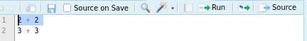
If we are writing code in a .R file, we have a few options. We could highlight the line we want to run, and use the “Run” button in the upper right hand corner of the scripts panel

Alternatively, the most common way of doing it, is to put your cursor on the chunk of code you want to run, or highlight the chunk, and then use a keyboard shortcut to run the code. On Mac computers, it’s usually Cmd+Return, and on Windows computers, it’s usually Ctrl+Enter. We can check what our shortcut is and/or change that shortcut to what we want, by going to the Keyboard Shortcuts menu:

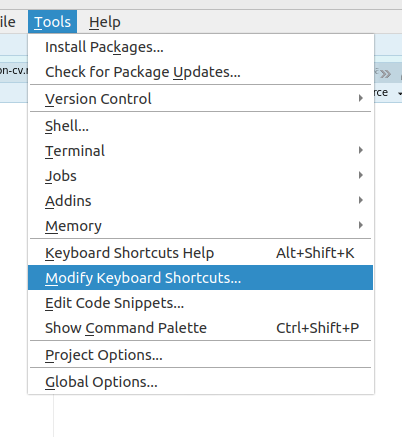
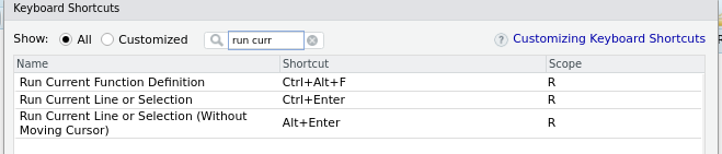
And then searching for the shortcut that does Run Current Line or Selection:

We can see that on my computer currently it’s Ctrl+Enter.

In an R Markdown

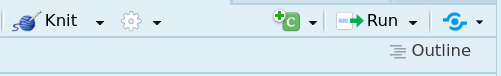
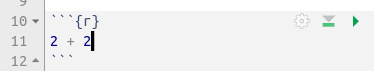
In an R Markdown document we have a few more options. To run code, first of all we have to open a code chunk, which can be done with the green “C” chunk button:

Or with a keyboard shortcut. On Windows this shortcut is Ctrl+Alt+I and on Mac it is Cmd+Option+I by default. Once we have the chunk of code, we have a number of ways we can run the code. First, we can just use our Ctrl+Enter method of before, or we can use the handy run button that RStudio provides for us:

Which is the little green play button icon on the right side.

Now that we know how to execute code, or essentially ask R to do things for us, we can continue our pathway of learning how to make R help us with our research!

---

Writing Comments

As you write R code, it’s incredibly helpful to leave notes for yourself and for others who might read your code in the future. These notes are called “comments.” R will ignore anything on a line that follows the # symbol (the hash or pound symbol). This means you can write explanations, reminders, or temporarily disable lines of code without R trying to execute them.

# This is a comment. R will ignore this entire line.

2 + 2 # This part is code, but the comment after the hash is ignored.

# print("This line is commented out, so it won't run")
print("This line will run!")

## [1] "This line will run!"

Good commenting makes your code much easier to understand, especially when you come back to it after a break!

R as a Calculator

At the most basic level, we can use R as a (very complicated) calculator. We can perform all the most basic operations that we might be interested in.

The classic operations (addition, subtraction, multiplication, division) work much as you might expect

    2 + 2

## [1] 4

    3 - 2

## [1] 1

    3 * 2 # multiplication is denoted by an asterisk

## [1] 6

    6 / 2

## [1] 3

    2 ^ 3 # exponentiation is denoted by this caret

## [1] 8

R also supports other useful arithmetic operations:

Modulo Operations

The modulo operation returns the remainder of a division, after one number is divided by another Getting the remainder of division:

    5 %% 2

## [1] 1

Integer Division

Only returns the integer value and not the decimal places:

    5 %/% 2

## [1] 2

Boolean Operations

We can ask R to make comparisons between values and give us a boolean (true or false) response for a wide variety of operations.

We can ask R if two values are equal ==, not equal !=, greater than >, less than <, greater than or equal to >=, or less than or equal to <= . Some examples:

    2 == 2

## [1] TRUE

    2 != 3

## [1] TRUE

    2 > 4

## [1] FALSE

Of note here is the difference between == and =. In R, == never performs any type of assignment, it only works to ask “are these two things equal to each other?”, whereas the = will assign a value to a variable.

Assignment

You’ll notice that up to now, we have simply been using numbers, but we can also use variables in R to store the values of numbers. If we wanted a variable x with value 2, we could assign this value in R using the assignment operator, <-. Once a variable is assigned, that variable will be stored in the environment, and can be called at any later point in the session.

    x <- 2
    x

## [1] 2

Two important notes with assignment:

1. In R, assignment can be done either through <- or =. Both will work identically, but the <- assignment operator is the more commonly used one and is technically best practice. Ideally, we should use <- to assign things (like objects and functions, which we’ll cover later) to variables, and then we can use = to pass arguments in expressions
2. If you make an assignment of a value to a variable, that assignment is not permanent. You can overwrite that assignment simply by using the same variable name

Built-in Functions

Most of your initial use of R will involve using built-in functions that R provides. For example, we might want to know the sum of a set of numbers.

    sum(1, 6, 8)

## [1] 15

Functions are discussed in more depth later, but generally, the way they work in R is by calling the word for the function (i.e. sum()) followed by a set of parentheses, which contain the function’s arguments. Arguments are simply a few items that the function needs to provide the right answer to the question.

One can always find what arguments are needed in the function by running `?` and then the function in question. For example,

    ?sum

This will not return anything to the console, but in the bottom right panel of RStudio, the help window will open, with the documentation on the function. For the ?sum example, the output is:

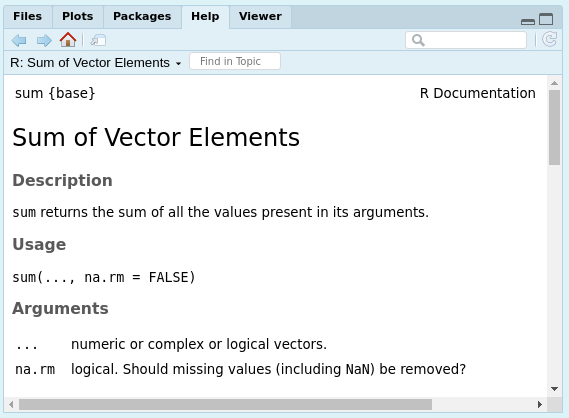
TIP: When in doubt about how to use a function, or really anything in R, check the documentation!

Naming

A lot of working with R involves assigning values to variables, and each of those variables will need a name. Many programming languages have “style guides” that are a generally agreed-upon set of standards by the community of users that dictate how best to do common tasks in that language.

There are a handful of suggested style guides in R, but the most common and the one followed in this resource is Hadley Wickham’s style guide , which is based on that of Google’s R style guide.

With respect to naming:

Variable and function names should be lowercase. Use an underscore (_) to separate words within a name. Generally, variable names should be nouns and function names should be verbs. Strive for names that are concise and meaningful (this is not easy!).

Important Note on Naming: R is case-sensitive. This means that my_variable, My_Variable, and MY_VARIABLE would all be treated as different, distinct variables by R. Be consistent with your capitalization to avoid confusion and errors!

Understanding Errors in R

Encountering errors is a normal and expected part of programming in R. Rather than being discouraged by errors, it’s helpful to view them as learning opportunities. R’s error messages are actually trying to help you understand what went wrong.

Here’s a common error you might encounter:

# This will produce an error
x + 5

# Error in x + 5 : object 'x' not found

This error message tells us exactly what went wrong: we tried to use a variable x that hasn’t been defined yet. To fix this, we need to assign a value to x first:

# This works
x <- 10
x + 5

# [1] 15

When you encounter an error in R:

• Read the error message carefully – It often contains valuable information about what went wrong
• Check your spelling and capitalization – R is case-sensitive, so Mean() and mean() are different
• Verify your variable names – Make sure you’ve defined all variables before using them
• Check your parentheses and brackets – Make sure they’re properly matched

Remember: Every programmer, no matter how experienced, encounters errors. The key is to:

• Stay calm and read the error message
• Break down complex operations into smaller steps
• Use R’s help system (?function_name) to check function usage
• Learn from each error – they’re opportunities to better understand how R works

Advanced – tryCatch()

Sometimes you want to handle errors programmatically rather than having them stop your code. The tryCatch() function allows you to specify what should happen when an error occurs. Here’s a basic example:

# Basic tryCatch example
result <- tryCatch(
  # Try to run this code
  {
    x <- 10
    y <- "not a number"
    x + y  # This will cause an error
  },
  # If an error occurs, run this code instead
  error = function(e) {
    message("An error occurred: ", e$message)
    return(NA)  # Return NA instead of stopping
  }
)

# The code continues running even though there was an error
print(result)  # [1] NA

Common uses for tryCatch() include:

• Handling missing or invalid data gracefully
• Providing alternative calculations when the primary method fails
• Logging errors for debugging without stopping the program
• Ensuring cleanup code runs even if an error occurs

Objects & OOP

To understand what’s going on in R, it’s important to understand how the things (termed “Objects”) are being stored in R. Everything (yes, literally everything) is an object. Objects are the basic building blocks in R. Think of an object as a named container that can hold data (like numbers or text) or even more complex things like entire datasets or models. We’ll learn about different types of objects as we go. For now, just remember that when you create something and give it a name in R, you’re creating an object. This concept is central to what is called object-oriented programming.

Object-oriented programming languages (sometimes called ‘high-level’ languages) are typically more intuitive and are often used via an IDE (integrated development environment) like RStudio or a GUI (graphical user interface).

Frequently Asked Questions

What’s the deal with the <- assignment operator?

In R, you can use either <- or = for assignment. Both are valid, but there are some conventions and subtle differences to be aware of:

# Both of these do the same thing - assign the value 5 to x
x <- 5
x = 5

# However, there are some differences in how they work in function calls
# This works as expected
mean(x = 1:10)

# This might not work as expected in some contexts
mean(x <- 1:10)  # This actually creates a new variable x!

The <- operator is the traditional R assignment operator and is generally preferred because:

• It’s more explicit about assignment vs. argument passing
• It’s the standard in R style guides
• It helps distinguish between assignment and equality testing (==)

Can I write the code in one line, or do I have to write it in different lines?

While R allows you to write code in a single line, it’s generally better to break it into multiple lines for readability. Here’s an example:

# This is valid but hard to read
result <- mean(sqrt(abs(sin(cos(tan(pi/4)))))) + sum(1:10) * max(c(1,2,3,4,5)) / min(c(1,2,3,4,5))

# The same code, broken into logical steps with some intermediate variables
# Calculate the trigonometric part
trig_part <- mean(sqrt(abs(sin(cos(tan(pi/4))))))

# Calculate the statistical part
stat_part <- sum(1:10) * max(c(1,2,3,4,5)) / min(c(1,2,3,4,5))

# Combine the results
result <- trig_part + stat_part

Some tips for clean code formatting:

• Break long lines at logical points (after operators, commas, etc.)
• Use consistent indentation (usually 2 or 4 spaces)
• Add spaces around operators for better readability
• Use intermediate variables for complex parts of your calculation

RStudio can help you format your code automatically. You can use the keyboard shortcut Ctrl+Shift+A (Windows/Linux) or Cmd+Shift+A (Mac) to format the selected code, or go to Code > Reformat Code in the menu.