Data Structures
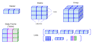
Previously we went over data types which refers to a single piece of data. To make use of these individual pieces of data we combine them together into data structures. Note that in R, individual data types (like numbers or text) as well as these more complex data structures, are all considered ‘objects’ once you assign them to a variable. When you make an assignment, and you see a new variable in your environment, that is an object! There are 4 main data structures that we work with consistently:
- Vectors
- Matrices
- DataFrames
- Arrays
This helpful graphic may help you cement these types in your memory
Vectors
Vectors can be divided into two main types: atomic vectors (which hold items of the same data type) and lists (which can hold items of different data types). Atomic vectors are the real workhorses in R, and most other object-oriented programming (OOP) languages use a similar structure for holding collections of data. From this point forward, we’ll use “vector” to refer to atomic vectors and call lists by name. We make vectors the same way we make variables, with an assignment statement.
Atomic Vectors
Often we start by making an empty vector that we may decide to fill with values later. To do this, we use the vector() function.
x <- vector("character", length = 5)Here, the function vector() takes two required arguments. The first argument asks for the data type we would like to use, and the second is the number of elements (the length) that we want the vector to be.
When we already know the content we want included, we can use a simpler c() function (c is short for combine).
x <- c(1, 2, 3, 4)Here, R automatically understands what type of data we’re using and since we passed four values, the length is automatically four. We could actually shorten this using R’s : notation:
y <- c(1:4)And we can check this works as expected:
x == y## [1] TRUE TRUE TRUE TRUENote: One thing to understand is that previously when we assigned a variable a single value (like a number or a piece of text), what R was actually doing is making a vector! This is just a special case where the vector length is 1.
We can determine what is and what is NOT an atomic vector by using the function is.atomic(). Recall that lists are technically a type of vector in R. However, when we talk about ‘atomic’ vectors, we mean vectors where all elements are of the same data type. The is.atomic() function specifically checks if an object is this kind of ‘all-same-type’ vector. This is important because the simpler is.vector() function will return TRUE for both atomic vectors and lists, so it doesn’t help us differentiate them. See here:
x <- list("a", "b", 1, 2)
is.vector(x)
## [1] TRUEWe can see that this returns TRUE. Since different methods can be applied to a list versus an atomic vector, it’s important to know which one we’re dealing with.
The structure of a vector, especially character vectors (strings), can differ significantly based on how you create it, which in turn affects how you can work with it. For example, here we have two vectors that spell out the same sentence, but are not equivalent:
  x  <- c("The quick brown fox jumped over the lazy dog")
  y <- c("The", "quick", "brown", "fox", "jumped", "over",
          "the", "lazy", "dog")
  x == y
## [1] FALSE FALSE FALSE FALSE FALSE FALSE FALSE FALSE FALSEWe can see by checking the length of each that their lengths are not equivalent. The second vector y is actually made up of 9 individual data pieces, while x is a singular datum:
length(x)## [1] 1 length(y)## [1] 9Vectors are flexible in that we can bind them together easily:
  x1 <- c(x, "who was sunning himself")
  y1 <- c(y, "who", "was", "sunning", "himself")
and also simply edit components of them:
  y[9] <- "cat"
  y
## [1] "The" "quick" "brown" "fox" "jumped" "over" "the"
## [8] "lazy" "cat"Note: We can only do this here because we created each word as its own data point inside the vector y. If we tried to modify part of the sentence in the vector x (which is a single string), it wouldn’t work in the same way because x is a single element. The above is an example of indexing which we discuss in the subsequent article, but for now, it can be interpreted as selecting an element of the vector and changing it.
Named Vectors
In R, you can assign names to the elements of a vector. This can make your code more readable and allows you to access elements by their name instead of only by their numerical index (which we’ll discuss in the Indexing & Querying section).
You can create a named vector when you define it, or add names to an existing vector.
# Creating a named vector at definition
fruit_prices <- c(apple = 0.5, banana = 0.25, orange = 0.75)
fruit_prices

# Accessing an element from a named vector using a name
fruit_prices["banana"]

# Another example with numeric data
student_scores <- c(John = 85, Lisa = 92, Peter = 78)
student_scores

# You can also use the names() function to add or get names
ages <- c(25, 30, 22)
names(ages) <- c("Alice", "Bob", "Charlie")
ages
ages["Alice"]
## apple banana orange
## 0.50 0.25 0.75
## banana
## 0.25
## John Lisa Peter
## 85 92 78
## Alice Bob Charlie
## 25 30 22
## Alice
## 25Lists
Lists are another type of vector, but with a key difference: they are more flexible because they can contain multiple data types within a single list, whereas atomic vectors require all elements to be of the same type. They are created much the same as vectors:
  l <- list(1, 2, "R is fun", c(1, 2, 3), TRUE)
  l
## [[1]]
## [1] 1
##
## [[2]]
## [1] 2
##
## [[3]]
## [1] "R is fun"
##
## [[4]]
## [1] 1 2 3
##
## [[5]]
## [1] TRUEHere we see a number of square brackets denoting the indexing of the list object l. This looks confusing but will be discussed in the Indexing & Querying section.
Instead of these numbers, we could name the list components. This is often handy for keeping data of variable lengths/types that can be related together. For example:
  eeb_prof <- list("name" = "Dr. Agrawal",
      "positions" = c("Distinguished Professor of Evolutionary Genetics",
              "Associate Chair, Graduate Studies"),
      "concentrations" = c("Genetics, Genomics & Molecular Evolution",
                    "Theoretical & Computational Biology"))

  eeb_prof
## $name
## [1] "Dr. Agrawal"
##
## $positions
## [1] "Distinguished Professor of Evolutionary Genetics"
## [2] "Associate Chair, Graduate Studies"
##
## $concentrations
## [1] "Genetics, Genomics & Molecular Evolution"
## [2] "Theoretical & Computational Biology"We now see we have three named list components, each of which gives a different piece of information about the professor at hand.
We will not work much with lists here as their primary utility does not become apparent until more advanced types of computations are required.
Matrices
Matrices are a logical extension of vectors as they can be thought of as a series of vectors bound together to form a 2D structure made up of rows and columns. Like atomic vectors, all elements within a single matrix must be of the same data type (e.g., all numeric or all character). They are also constructed similarly:
  m <- matrix(nrow = 2, ncol = 2)
  m
## [,1] [,2]
## [1,] NA NA
## [2,] NA NAThis above is an empty matrix, we haven’t told R to put anything in the matrix, but this empty matrix concept is used frequently to preallocate memory before being filled in later. We could make a matrix with some values like this:
m <- matrix(100, nrow = 2, ncol = 2)And this will make a matrix with four values of 100. Multiple values are possible as well:
m <- matrix(c(100, 200, 300, 400), nrow = 2, ncol = 2)Here we passed an atomic vector as the first argument to matrix(), and then the dimensions that we wanted to get for our matrix. Note that if the number of elements in the vector passed to matrix() is not an exact multiple of the number of rows (or columns, depending on how R fills the matrix by default or if byrow=TRUE is used), R will typically recycle the vector elements to fill the matrix. However, if the length of the input vector is not compatible with the nrow * ncol product (e.g., trying to fill a 3×2 matrix with 4 elements), you will get a warning, and the matrix might not be what you expect. Try running the following code in your R console and see what output you get:
m <- matrix(c(100, 200, 300, 400), nrow = 3, ncol = 2)We can also make matrices by combining existing vectors. Let’s make two vectors and combine them into a matrix using two different approaches:
  vec1 <- c(1, 2)
  vec2 <- c(3, 4)
First, if I want vec1 to be the first row and vec2 to be the second row, I simply need to bind them together as rows with the aptly named rbind() function:
  m1 <- rbind(vec1, vec2)
  m1
## [,1] [,2]
## vec1 1 2
## vec2 3 4If instead I wanted vec1 to be the first column and vec2 to be the second column, I would bind them together as columns using the cbind() function:
  m2 <- cbind(vec1, vec2)
  m2
## vec1 vec2
## [1,] 1 3
## [2,] 2 4DataFrames
The darlings of R. These structures are the feature of R that make it so popular for data analysis and statistics. It is the easiest way to store, access, and perform operations on tabular data (the type of data we most often have in biology). Dataframes are actually a type of list, one wherein each element of the list has the same length, making it of dimension 2, which means we easily can look at rows and columns. They’re usually created directly by reading in data from files (a topic covered in more detail elsewhere), or by constructing them manually using the data.frame() function:
  c1 <- c(1:4)
  c2 <- c("item1", "item2", "item3", "item4")
  c3 <- c(11:14)

  # we can combine these values as columns into a dataframe
  d <- data.frame(c1, c2, c3)
  d
## c1 c2 c3
## 1 1 item1 11
## 2 2 item2 12
## 3 3 item3 13
## 4 4 item4 14It’s easy to add rows or columns using column binding, which is done with the cbind() function:
  c4 <- c("add1", "add2", "add3", "add4")
  d1 <- cbind(d, c4)
  d1
## c1 c2 c3 c4
## 1 1 item1 11 add1
## 2 2 item2 12 add2
## 3 3 item3 13 add3
## 4 4 item4 14 add4Or row binding, performed with the rbind() function:
  r5 <- list(5L, "item5", 15L, "add5")
  d2 <- rbind(d1, r5)
  d2
## c1 c2 c3 c4
## 1 1 item1 11 add1
## 2 2 item2 12 add2
## 3 3 item3 13 add3
## 4 4 item4 14 add4
## 5 5 item5 15 add5Notice above to create row 5, we used list() instead of c(). Why? Recall that c() only works for atomic vectors, so if we used the same arguments but the command c(), R would think we wanted an atomic vector, so would actually change our integer values to characters. Let’s look at it:
  r5_char <- c(5L, "item5", 15L, "add5") # Using c() would create a character vector
  r5_char
## chr [1:4] "5" "item5" "15" "add5"We can see all the values of r5_char are now characters. This is why list() was used for r5 when originally creating d2, to preserve the intended data types for each column before binding.
Also, notice in the r5 <- list(5L, "item5", 15L, "add5") example, we used 5L and 15L to explicitly create integers. If we had used list(5, "item5", 15, "add5") (let’s call this r5_numeric_list), R would have interpreted 5 and 15 as numeric (double) by default. When this list is then row-bound (rbind) to a dataframe (like d1) where the corresponding columns c1 and c3 were originally integers, R would convert the entire columns c1 and c3 to numeric to maintain type consistency within each column. This is because a column cannot hold mixed types like integers and numerics simultaneously; R will coerce them to the more general type (numeric, in this case). Let’s see the structure of such a list:
  r5_numeric_list <- list(5, "item5", 15, "add5")
  str(r5_numeric_list)
## List of 4
## $ : num 5
## $ : chr "item5"
## $ : num 15
## $ : chr "add5"Note that the first and third elements in r5_numeric_list now have type num instead of type int!
  d3 <- rbind(d1, r5_numeric_list) # d1 had c1 and c3 as integers
  d3
## c1 c2 c3 c4
## 1 1 item1 11 add1
## 2 2 item2 12 add2
## 3 3 item3 13 add3
## 4 4 item4 14 add4
## 5 5 item5 15 add5If we inspect d3 (created with r5_numeric_list that used non-L numbers), we would see that columns c1 and c3 are now of numeric (double) type (you can verify this with str(d3)). This isn’t necessarily a big deal for many calculations, as integers and numerics are often treated similarly, but it’s something to be aware of if you strictly need a column to remain integer type.
Dataframes are ultra-flexible, and have a lot of underlying structure. The best way to inspect this structure is with the str() command (here showing str(d2) which was made correctly with r5 using L):
str(d2)## 'data.frame': 5 obs. of 4 variables:
## $ c1: int 1 2 3 4 5
## $ c2: chr "item1" "item2" "item3" "item4" "item5"
## $ c3: int 11 12 13 14 15
## $ c4: chr "add1" "add2" "add3" "add4" "add5"We can also get the column names of a dataframe with the names() function:
names(d2)## [1] "c1" "c2" "c3" "c4"the number of rows or columns with the nrow() and ncol() functions, respectively:
nrow(d2)## [1] 5 ncol(d2)## [1] 4or a summary of the dataframe with the summary() function:
summary(d2)## c1 c2 c3 c4
## Min. :1 Length:5 Min. :11 Length:5
## 1st Qu.:2 Class :character 1st Qu.:12 Class :character
## Median :3 Mode :character Median :13 Mode :character
## Mean :3 Mean :13
## 3rd Qu.:4 3rd Qu.:14
## Max. :5 Max. :15For the integer columns, we get a very helpful summary of the values in the column.
Factors
We will briefly discuss factors here as their most common use is as columns in dataframes. Factors are variables which can only take on a certain number of values (aka “levels”). They are often referred to as the “categorical” variables of R. They are of special importance in statistical modelling since categorical variables enter into statistical models in a different way than continuous variables may do.
Similar to other datatypes, they can be created with their own function:
  fac <- factor(c("one", "two", "three", "four", "one", "two", "three", "four"))
  fac
## [1] one two three four one two three four
## Levels: four one three twoThe output here shows the values we passed (those within the c() function), but the levels aren’t what we might expect. We passed strings that represent numbers (“one”, “two”, etc.), but R treats them purely as text strings and, by default, orders the levels alphabetically. We can control the order of factors with an additional argument to the function factor():
  fac1 <- factor(c("one", "two", "three", "four", "one", "two", "three", "four"),
                levels = c("one", "two", "three", "four"))
  fac1
## [1] one two three four one two three four
## Levels: one two three fourNow the levels are in a more logical order.
Factors are most commonly used in dataframes, so let’s change one of our chr variables in a dataframe we’ve already made to a factor.
d## c1 c2 c3
## 1 1 item1 11
## 2 2 item2 12
## 3 3 item3 13
## 4 4 item4 14Currently d2 has c2 column of type chr, but let’s make it a factor. We could do this by changing the way we define c2 originally like this:
  c1 <- c(1:4)
  c2 <- factor(c("item1", "item2", "item3", "item4"))
  c3 <- c(11:14)

  # we can combine these values as columns into a dataframe
  d <- data.frame(c1, c2, c3)
  d
## c1 c2 c3
## 1 1 item1 11
## 2 2 item2 12
## 3 3 item3 13
## 4 4 item4 14But often we want to perform “in-place” operations to dataframes already created, so let’s create the dataframe as before then once created, only re-create that one column:
  c1 <- c(1:4)
  c2 <- c("item1", "item2", "item3", "item4")
  c3 <- c(11:14)

  # we can combine these values as columns into a dataframe
  d <- data.frame(c1, c2, c3)
  d
## c1 c2 c3
## 1 1 item1 11
## 2 2 item2 12
## 3 3 item3 13
## 4 4 item4 14So currently it’s a chr, but we can index our column of interest by name, using the $ operator, and perform the change this way. To change the column to a factor we again can use the factor() column:
  d$c2 <- factor(d$c2)
  str(d)
## 'data.frame': 4 obs. of 3 variables:
## $ c1: int 1 2 3 4
## $ c2: Factor w/ 4 levels "item1","item2",..: 1 2 3 4
## $ c3: int 11 12 13 14Now we can see from the str(d) output that c2 is a Factor column. More on indexing here.
Ordinal Factors
In addition to standard factors, R allows for ordinal factors. These are used when the levels of a factor have a natural ordering or ranking. For example, responses to a survey question like “low”, “medium”, “high” have a clear order, unlike nominal categories such as “red”, “green”, “blue” where order doesn’t inherently matter.
Knowing that there’s an order to the levels can be important for some types of statistical analysis and for visualizations, as R can then treat the levels appropriately according to their rank.
You create an ordinal factor by using the same factor() function, but with an additional argument: ordered = TRUE. You should also explicitly provide the levels argument in their correct order.
# Example: T-shirt sizes
sizes <- c("M", "S", "L", "M", "S", "XL", "S", "L")

# Create an ordinal factor
ordered_sizes <- factor(sizes,
                        ordered = TRUE,
                        levels = c("S", "M", "L", "XL"))

ordered_sizes
str(ordered_sizes)
summary(ordered_sizes)
## [1] M S L M S XL S L
## Levels: S < M < L < XL
## Ord.factor w/ 4 levels "S"<"M"<"L"<"XL": 2 1 3 2 1 4 1 3
## S M L XL
## 3 2 2 1 Notice the output of ordered_sizes now shows the levels with < signs between them (e.g., S < M < L < XL), indicating their order. The str() output also identifies it as an Ord.factor.
# Comparing elements from an ordinal factor
ordered_sizes[1] > ordered_sizes[2] # Is Medium > Small?
## [1] TRUEBecause the factor is ordered, you can now make logical comparisons like ordered_sizes[1] > ordered_sizes[2], which correctly evaluates to TRUE because “M” is ordered higher than “S”. Such comparisons would not be meaningful (and might produce warnings or errors) with standard (nominal) factors.
Tibbles
Tibbles are useful to go over since a number of very common packages make heavy use of this data structure. A tibble is a “modern reimagining of the data.frame”; they are very similar, but with some key differences in how they behave (e.g., printing, subsetting, and handling of column names). You can learn more here if you’re interested.
Arrays
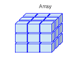
Lastly, we’ll look at arrays. Arrays generalize vectors and matrices to potentially more than two dimensions. While they can be difficult to visualize when they have more than two dimensions (e.g., 3D, 4D, etc.), let’s focus on a 3-dimensional example for now. Again, we can create an array with the array() function, combining multiple vectors.
  vec1 <- c(1, 2, 3)
  vec2 <- c(4, 5, 6)
  vec3 <- c(7, 8, 9)
  ar1 <- array(c(vec1, vec2, vec3), dim = c(3, 3, 2))
  ar1
## , , 1
##
## [,1] [,2] [,3]
## [1,] 1 4 7
## [2,] 2 5 8
## [3,] 3 6 9
##
## , , 2
##
## [,1] [,2] [,3]
## [1,] 1 4 7
## [2,] 2 5 8
## [3,] 3 6 9The input vector c(vec1, vec2, vec3) has 9 elements. Since our array ar1 is defined with dim = c(3,3,2), it requires 3*3*2 = 18 elements. R recycles the values from the input vector to fill the array, which is why the second matrix (, , 2) is identical to the first in this example.
We can read the dims argument just as we would order mathematical dimensions, always starting with x the first dimension, `y`, the second, and then z the third one. So we can think of this as having three rows (the x coordinate), and three columns (the y coordinate), which make up a single matrix in each of the two z dimensions. It’s helpful to visualize this:
It’s often helpful to name each of our columns, rows, and matrices. To do this for the above array we might do the following:
  row_names <- c("row1", "row2", "row3")
  col_names <- c("col1", "col2", "col3")
  mat_names <- c("mat1", "mat2")

  # now remake the array with the names
  ar_named = array(c(vec1, vec2, vec3), dim = c(3, 3, 2),
                  dimnames = list(row_names, col_names, mat_names))
  ar_named
## , , mat1
##
## col1 col2 col3
## row1 1 4 7
## row2 2 5 8
## row3 3 6 9
##
## , , mat2
##
## col1 col2 col3
## row1 1 4 7
## row2 2 5 8
## row3 3 6 9With the rows, columns, and matrices now named it’s easier to refer to them.
Conclusion
Understanding R’s fundamental data structures – Vectors, Lists, Matrices, DataFrames, and Arrays – is crucial for effective data manipulation and analysis. Each structure has its own strengths and is suited to different types of data and tasks.
Vectors form the building blocks, with atomic vectors holding elements of the same type and named vectors providing more descriptive access. Lists offer flexibility by allowing elements of different types. Matrices extend vectors into two dimensions for homogenous data, while DataFrames, the workhorse of R, provide a tabular structure ideal for datasets with columns of varying types, including specialized Factor columns for categorical data (both nominal and ordinal). Finally, Arrays generalize these structures to multiple dimensions.