Indexing Objects

Vectors

Vectors are indexed via the [] notation. In a one-dimensional vector, the simplest and most common way to index is to pass the index or element number we want to those square brackets.

x <- c(1, 3, 9, 10, 76, 89)

If we want to index the 9 in this vector, that’s in the third position, or index 3.

x[3]

## [1] 9

Similarly with a character vector

y <- c("The", "quick", "brown", "fox", "jumped", "over", "the", "lazy", "dog")

If we want to access the element “fox”, the fourth element, we will write:

y[4]

## [1] "fox"

While indexing vectors, we can also return all the elements of a vector NOT in a certain position via the `-` sign:

y[-1]

## [1] "quick"  "brown"  "fox"    "jumped" "over"   "the"    "lazy"  
## [8] "dog"

This returns all the elements of the vector except the first one.

We can also index based on multiple positions by providing a vector of indices inside the square brackets:

y[c(1, 4, 9)] # c(1, 4, 9) creates a vector of desired indices

## [1] "The" "fox" "dog"

This returns the first, fourth, and ninth elements.

Indexing Named Vectors

If a vector has names, you can also access its elements using their names, either individually or by providing a vector of names. This often makes code more readable.

# From Data_Structures.md example:
fruit_prices <- c(apple = 0.5, banana = 0.25, orange = 0.75)

# Accessing a single element by name
fruit_prices["banana"]

# Accessing multiple elements by a vector of names
fruit_prices[c("orange", "apple")]

# This also works for assignment
fruit_prices["banana"] <- 0.30
fruit_prices

## banana
##   0.25
## orange  apple
##   0.75   0.50
## apple banana orange 
##  0.50   0.30   0.75

Lists

Since lists are also vectors, they’re also indexed with similar notation, but it’s crucial to understand the distinction between [] and [[]]. Recall that each element of a list can itself be another object (a vector, another list, a dataframe, etc.).

• Using single square brackets [] to index a list will always return a new list (a sub-list) containing the selected elements.
• Using double square brackets [[]] to index a list extracts the actual element itself from the list. You can only use [[]] to extract a single element.

Let’s illustrate:

l <- list(item1 = 1, item2 = "R is fun", item3 = c(10, 20, 30), item4 = TRUE)

# Using single brackets [] - returns a list
sub_list_one_element <- l[3] 
print("Output of l[3]:")
sub_list_one_element
str(sub_list_one_element)

sub_list_multiple_elements <- l[c(1,3)]
print("Output of l[c(1,3)]:")
sub_list_multiple_elements
str(sub_list_multiple_elements)

# Using double brackets [[]] - extracts the element
extracted_element <- l[[3]]
print("Output of l[[3]]:")
extracted_element
str(extracted_element)

# You can also use names with [[]]
print("Output of l[['item2']]:")
l[['item2']]

# Accessing an element within an extracted list element
print("Output of l[[3]][2]:")
l[[3]][2] # Access the second value of the vector stored in item3

# Reassigning a value within an extracted list element
l[[3]][2] <- 25
print("List l after l[[3]][2] <- 25:")
l

## [1] "Output of l[3]:"
## $item3
## [1] 10 20 30
## List of 1
##  $ item3: num [1:3] 10 20 30
## [1] "Output of l[c(1,3)]:
## $item1
## [1] 1
## $item3
## [1] 10 20 30
## List of 2
##  $ item1: num 1
##  $ item3: num [1:3] 10 20 30
## [1] "Output of l[[3]]:"
## [1] 10 20 30
##  num [1:3] 10 20 30
## [1] "Output of l[['item2']]:"
## [1] "R is fun"
## [1] "Output of l[[3]][2]:"
## [1] 20
## [1] "List l after l[[3]][2] <- 25:"
## $item1
## [1] 1
## 
## $item2
## [1] "R is fun"
## 
## $item3
## [1] 10 25 30
## 
## $item4
## [1] TRUE

In the example l[[4]][3] <- 5 from before (if l was list(1, 2, "R is fun", c(1, 2, 3), TRUE)), l[[4]] extracts the fourth element (the vector c(1,2,3)), and then [3] accesses the third element of that extracted vector for reassignment.

If we recall, we can also have named lists, which can be indexed by their names.

agrawal <- list("name" = "Dr. Aneil Agrawal",
                "positions" = c("Distinguished Professor of Evolutionary Genetics",
                                "Associate Chair, Graduate Studies"),
                "concentrations" = c("Genetics, Genomics & Molecular Evolution",
                                        "Theoretical & Computational Biology"))
names(agrawal)

## [1] "name"           "positions"      "concentrations"

By calling names() we can see the names of the different list components. We can index by any of these names.

# Using single brackets [] with a name returns a sub-list
agrawal["concentrations"]
str(agrawal["concentrations"])

## $concentrations
## [1] "Genetics, Genomics & Molecular Evolution"
## [2] "Theoretical & Computational Biology"
## List of 1
##  $ concentrations: chr [1:2] "Genetics, Genomics & Molecular Evolution" "Theoretical & Computational Biology"

Alternatively, the $ operator or double square brackets [[]] with a name can be used to extract the element directly:

# Using $ to extract the element directly
agrawal$concentrations
str(agrawal$concentrations)

# Using [[]] with a name also extracts the element directly
agrawal[["concentrations"]]
str(agrawal[["concentrations"]])

## [1] "Genetics, Genomics & Molecular Evolution"
## [2] "Theoretical & Computational Biology"
##  chr [1:2] "Genetics, Genomics & Molecular Evolution" "Theoretical & Computational Biology"
## [1] "Genetics, Genomics & Molecular Evolution"
## [2] "Theoretical & Computational Biology"
##  chr [1:2] "Genetics, Genomics & Molecular Evolution" "Theoretical & Computational Biology"

This provides the same direct output of the element’s contents. Now let’s say we wanted to access the second element in this “concentrations” vector. We could use the [[]][] notation, or the more common combination of $ and []:

agrawal$concentrations[2]

## [1] "Theoretical & Computational Biology"

Now let’s reassign it:

agrawal$concentrations[2] <- "Computational & Theoretical Biology"

To check if it worked print the `agrawal` list to our console:

agrawal

## $name
## [1] "Dr. Aneil Agrawal"
## 
## $positions
## [1] "Distinguished Professor of Evolutionary Genetics"
## [2] "Associate Chair, Graduate Studies"               
## 
## $concentrations
## [1] "Genetics, Genomics & Molecular Evolution"
## [2] "Computational & Theoretical Biology"

And we see it worked.

Matrices

Indexing matrices is simple as it is a 2-dimensional extension of indexing atomic vectors.

m <- matrix(c(100, 200, 300, 400), nrow = 2, ncol = 2)
m

##      [,1] [,2]
## [1,]  100  300
## [2,]  200  400

To access the value 300, we will need to specify that we want the value in the first row, and second column. Indexing in R is always done row then column.

m[1,2]

## [1] 300

We can get the entirety of the first row

m[1, ]

## [1] 100 300

or the first column

m[ ,1]

## [1] 100 200

by writing leaving the row/column argument empty, which tells R that for either condition, to include all values of that dimension. Note: When you extract a single row or a single column from a matrix in this way, R, by default, simplifies the result to a vector (it drops the matrix dimension). If you need to keep the result as a 1-row or 1-column matrix, you can use the drop = FALSE argument (e.g., m[1, , drop = FALSE]).

DataFrames

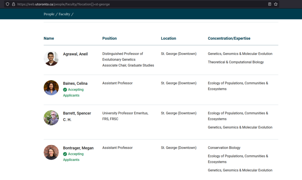
Dataframes are lists (a special kind wherein all the elements are of the same length), so their indexing is actually very similar. Let’s create an extension of the example we had above using some professors from the EEB department at the University of Toronto. We’ll make a dataframe combining the information for a number of categories.

This is just for fun, so let’s use the EEB website to get information on each of the professors’ names, the school they got their PhD at, and whether or not they’re accepting applicants for graduate work.

However, note that differently from above, we cannot have the “positions” nor the “concentrations” categories be of different lengths as that would violate the rules of a dataframe, so instead each category will be it’s own vector:

# first make a series of vectors, one for each intended column
names_vec <- c("Dr. Aneil Agrawal", "Dr. Celina Baines", "Dr. Spencer C.H. Barrett",
        "Dr. Megan Bontrager")
phd_vec <- c("Indiana", "Toronto", "Reading", "UBC")
accepting_vec <- c(FALSE, TRUE, FALSE, TRUE)


# now make a dataframe out of these vectors
prof_df = data.frame(names = names_vec, phd = phd_vec, accepting = accepting_vec)
prof_df

##                      names     phd accepting
## 1        Dr. Aneil Agrawal Indiana     FALSE
## 2        Dr. Celina Baines Toronto      TRUE
## 3 Dr. Spencer C.H. Barrett Reading     FALSE
## 4      Dr. Megan Bontrager     UBC      TRUE

If want to access any of the columns of this dataframe, we can do so by their names. Similar to lists, you can use the $ operator, or double square brackets [[]] for extracting a column as a vector. Single square brackets [] with a column name will return a dataframe containing just that column.

# Using $ to extract the column as a vector
prof_df$phd

# Using [[]] with a name to extract the column as a vector
prof_df[["phd"]]

# Using [] with a name returns a dataframe with one column
prof_df["phd"]
str(prof_df["phd"]) # Note the output is a data.frame

# You can also select columns by numeric index with [] or [[]]
prof_df[[2]] # Extracts the 2nd column (phd) as a vector
prof_df[2]   # Returns a dataframe containing the 2nd column

## [1] "Indiana" "Toronto" "Reading" "UBC"
## [1] "Indiana" "Toronto" "Reading" "UBC"
##       phd
## 1 Indiana
## 2 Toronto
## 3 Reading
## 4     UBC
## 'data.frame':	4 obs. of  1 variable:
##  $ phd: chr  "Indiana" "Toronto" "Reading" "UBC"
## [1] "Indiana" "Toronto" "Reading" "UBC"
##       phd
## 1 Indiana
## 2 Toronto
## 3 Reading
## 4     UBC

We could also look at a single row (which returns a dataframe):

prof_df[3, ]

##                      names     phd accepting
## 3 Dr. Spencer C.H. Barrett Reading     FALSE

which tells us all about Dr. Barrett. We could also ask whether or not the fourth row professor, Dr. Bontrager, is accepting students:

prof_df$accepting[4]

## [1] TRUE

Arrays

Since these are three dimensional objects, we must include all indices to get to a specific element. Let’s used the named array we had in the data structures section as our example here:

# pre-define the vectors
vec1 <- c(1, 2, 3)
vec2 <- c(4, 5, 6)
vec3 <- c(7, 8, 9)

# define the rownames 
row_names <- c("row1", "row2", "row3")
col_names <- c("col1", "col2", "col3")
mat_names <- c("mat1", "mat2")

# now remake the array with the names
ar_named = array(c(vec1, vec2, vec3), dim = c(3, 3, 2),
                dimnames = list(row_names, col_names, mat_names))
ar_named

## , , mat1
## 
##      col1 col2 col3
## row1    1    4    7
## row2    2    5    8
## row3    3    6    9
## 
## , , mat2
## 
##      col1 col2 col3
## row1    1    4    7
## row2    2    5    8
## row3    3    6    9

Note on Array Filling: The input vector c(vec1, vec2, vec3) has 9 elements. Since our array ar_named is defined with dim = c(3, 3, 2), it requires 3*3*2 = 18 elements. R recycles the values from the input vector to fill the array, which is why the second matrix (mat2) is identical to the first in this example.

To access elements, we use [row, column, matrix_layer]. So to see all rows and columns of just the second matrix (mat2), we write:

ar_named[,,2]

##      col1 col2 col3
## row1    1    4    7
## row2    2    5    8
## row3    3    6    9

but to see each of the second columns in both matrices and all rows, we can write:

ar_named[, 2, ]

##      mat1 mat2
## row1    4    4
## row2    5    5
## row3    6    6

Further, if we want only the first row and the third column elements for all matrices, we can write:

ar_named[1, 3, ]

## mat1 mat2 
##    7    7

but the value for the third row, first column, only in matrix 2 would be found by:

ar_named[3, 1, 2]

## [1] 3

A common use case is that we may want, rather than to index a position, tell our object to return to us some part of that object containing a particular value. This is called data filtering and is discussed here.

Conclusion

Effectively accessing and manipulating elements within R’s data structures is a fundamental skill. This article covered the primary methods for indexing vectors (including named vectors), lists, matrices, dataframes, and arrays. Key techniques include using single square brackets [] for basic subsetting (often returning a structure of the same type or a simplified vector), double square brackets [[]] for extracting individual elements (especially from lists and dataframes), and the $ operator for convenient named element access in lists and dataframes. Remember that R is 1-indexed, and understanding how dimensions are handled (e.g., [row, col] for 2D structures) is crucial. While this article focused on direct access by position or name, these indexing skills form the basis for more advanced data querying and filtering operations vital for data analysis.