Packages
Packages are essential to the work we do in R. Whether you are using R for the first time, or you’re a seasoned R expert, using packages makes up a great deal of your daily workload in R. It’s important to be familiar with the concept of a package, how we go about using them, and what to do when they don’t work how we want them to.
What are Packages?
R packages are collections of related functions, code, and data, which can be downloaded and used by any R user, as a way of avoiding having to write all the code to do a task manually ourselves. Think of installing a package like adding a new app to your phone – you do it once to get the software onto your device. Then, each time you want to use that app in a particular work session, you open or “load” it. Similarly, in R, you install a package once to download it to your computer. Then, in each R session where you want to use its functions, you load it using the library() command.
All official packages are submitted and verified through CRAN (Comprehensive R Archive Network). Packages typically are sets of functions that perform related tasks (e.g. data management). For example, if in an R script or .Rmd file, we begin to type the function subset(), we get the following:
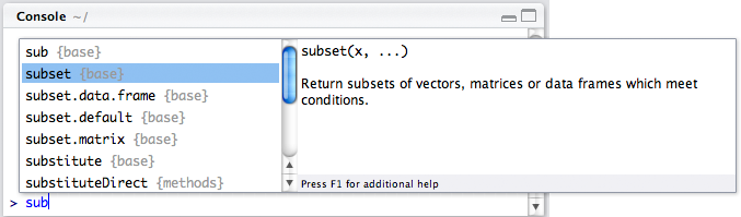
We see here that R is suggesting some options to us of functions that start with sub. The word in the curly braces, {base} indicates that that function is native to “base” R, or the base set of functions and methods that we have access to without loading in other packages. When you download R, a set of packages are imported automatically, including base, stats, and some others. Packages not downloaded automatically with R need to be explicitly loaded separately.
In fact, if you’ve opened R and read in some data, it’s likely you’ve already used a package! There are a set of packages that are standard (base) and ship with R when you install it on your computer. These packages are always automatically loaded and available for your use, so when you use a function that exists natively in R, such as the mean() function, that actually exists in a package that R loaded for you already.
There are many many packages, the vast majority of which we will not even talk about. In fact, as of November 2020, more than 16,000 packages were available on CRAN (and that’s not including the non-CRAN packages that are available too!).
Note that many packages are termed dependencies, that is, they are not the packages we are going to use directly, but they are required on our computers, for the package we do want to use to work properly. When you install a package using install.packages(), R will usually automatically download and install its dependencies as well, which is very helpful!
Installing Packages
Before installing new packages, you might want to see which packages are already available in your R environment or what you have installed. The library() command, when called without arguments, lists the packages in the default library locations (your R search path). This can give you an idea of what’s readily accessible.
library()The output will show a list of packages. If you want a more comprehensive list of all packages installed on your computer, including those not in the default search paths, the installed.packages() function is more direct. It returns a matrix with details about all installed packages.
# To see the first few rows of the installed packages matrix
head(installed.packages()[, c("Package", "Version", "LibPath")])
## Package Version LibPath
## base "base" "4.2.2" "/usr/lib/R/library"
## boot "boot" "1.3-28" "/usr/lib/R/library"
## class "class" "7.3-20" "/usr/lib/R/library"
## cluster "cluster" "2.1.4" "/usr/lib/R/library"
## codetools "codetools" "0.2-18" "/usr/lib/R/library"
## compiler "compiler" "4.2.2" "/usr/lib/R/library"This shows the package name, version, and where it’s located. On your computer, this list might be much longer or shorter, and that’s perfectly fine.
The EEB R Manual will make use frequently of packages that are part of the Tidyverse. One of the first packages we’ll use is the dplyr package, a very common and useful data cleaning package.
Installing Packages from CRAN
The Tidyverse
The Tidyverse is “…an opinionated collection of R packages designed for data science. All packages share an underlying design philosophy, grammar, and data structures” that is funded and developed by a company called Posit, which was previously known as the RStudio Foundation. It is a good resource for those learning R, as there are a ton of educational resources available
Okay, let’s install the package. Anytime we install a package we call install.package(), and put our package name inside quotations between the brackets.
install.packages("dplyr")## Installing package into '//home/user/R/x86_64-pc-linux-gnu-library/4.2'
## (as 'lib' is unspecified)
## trying URL 'https://cloud.r-project.org/src/contrib/dplyr_1.1.2.tar.gz'
## Content type 'application/x-gzip' length 1034591 bytes (1010 KB)
## ==================================================
## downloaded 1010 KB
##
## * installing *source* package 'dplyr' ...
## ** package 'dplyr' successfully unpacked and MD5 sums checked
## ** using staged installation
## ** R
## ** inst
## ** byte-compile and prepare package for lazy loading
## ** help
## *** installing help indices
## ** building package indices
## ** testing if installed package can be loaded from temporary location
## ** testing if installed package can be loaded from final location
## ** DONE (dplyr)
##
## The downloaded source packages are in
## '/tmp/RtmpXXXXXX/downloaded_packages'We see here a long output as the package installs and tells us how the process is going. We don’t need to worry too much about the specifics of this output, but the end part, where it tells us that The downloaded source packages are in … tells us that the installation process worked, and the software now exists on our computer. This process is the same for any new package we want.
Red Text while installing
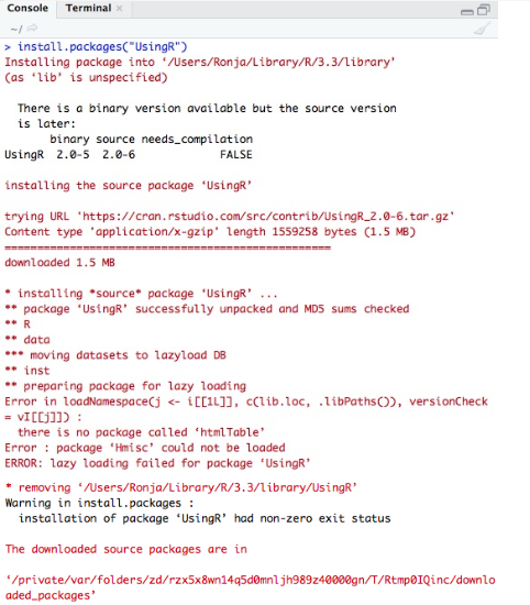
Particularly when using RStudio, the installation of packages typically features log messages that are red.
Red text doesn’t always mean failure. Sometimes it’s just a warning, note, or “important” (from the developer’s P.O.V) message.
On the right is an example of when it is a failure, as indicated by the uppercase ERROR message.
In other words, keep calm and read the output to ascertain whether an error truly occurred.
Installing Packages from Bioconductor (BiocManager)
Beyond CRAN, another major repository for R packages, especially those used in bioinformatics and for the analysis of high-throughput genomic data, is Bioconductor. Packages from Bioconductor are managed using a special package called BiocManager.
First, you need to install BiocManager itself from CRAN, if you haven’t already. You only need to do this once per R installation:
install.packages("BiocManager")Once BiocManager is installed, you can use its install() function to install packages from Bioconductor, CRAN, or even GitHub. For example, to install a Bioconductor package called “GenomicRanges” and a CRAN package “dplyr” at the same time:
BiocManager::install(c("GenomicRanges", "dplyr"))Bioconductor packages work best when they are all from the same release. BiocManager helps ensure this. You can check if your installed packages are up-to-date and valid for your Bioconductor version using:
BiocManager::valid()To update all your Bioconductor (and CRAN) packages to their current versions, you can run:
BiocManager::install()This will prompt you if there are updates available. For more detailed information on using BiocManager, refer to the official BiocManager vignette.
Installing Packages from Other Sources (e.g., GitHub)
While CRAN and Bioconductor are the primary repositories, sometimes you might need to install a package directly from other sources, like GitHub. This is often the case for packages under active development or those not yet submitted to CRAN. To do this, you typically use a function from the remotes or devtools packages. First, you’d install one of those, for example, install.packages("remotes"). Then, you can install a GitHub package using a command like remotes::install_github("username/repository_name"), replacing username/repository_name with the specific GitHub path for the package.
Loading a Package
Now that the package has been installed, we generally don’t need to call install.packages() for that specific package again on the same computer, unless you need to update it to a newer version or reinstall it for some reason. But, if we’ve just started an R session and we want to use the package, we’ll need to load it. That is, we want to tell R that we want to use the functions inside the package for our current R session. We do this via the library() function. We only need to call the library() call once in an R session for each package we want to use. If we load the library and then close R and re-start it, we’ll need to call library() again for that package in the new session.
As we discuss in the workflow section, it’s best to call all the packages that you want to use at the top of your script. Why? Well, R works its way through a script from top to bottom. So if we try to use a function in a package before we’ve actually called it, we’ll get an error. Let’s load the dplyr package now:
library(dplyr)##
## Attaching package: 'dplyr'## The following objects are masked from 'package:stats':
##
## filter, lag## The following objects are masked from 'package:base':
##
## intersect, setdiff, setequal, unionThere is some important information here in this library load. First of all, we see that two packages, package:stats and package:base now have “masked objects”. The objects that are masked for each of these packages are listed. For stats, filter() and lag() are masked, and for base, the functions intersect(), setdiff(), setequal(), and union() are masked.
Don’t worry, you don’t have to do anything about this, but just know that **this means there are functions in the dplyr package with the same names (i.e. filter() and lag(), and intersect(), setdiff(), setequal(), and union()) as functions that were already loaded in R. So, if you just call the function filter() it will default to using the function named filter() from the dplyr package, and NOT from the stats package.
It is good practice to be explicit about what package you are using for what task with thepackage::function() notation. That is, if I wanted to use the filter() function from dplyr, I would write: dplyr::filter(), but if I wanted to use the function from the stats package I would write stats::filter(). This way R will not get confused and perhaps default to the wrong package!
Understanding Namespace Clashing and Using ::
As you start using more packages, you might encounter situations where different packages have functions with the same name. This is known as “namespace clashing” or “masking.” Each R package has its own namespace, which is like a container that holds all its functions and objects. When you load a package with library(), R makes its functions available. If you load a package that has a function with the same name as a function in an already loaded package (or in base R), the newly loaded package’s function will “mask” or hide the previous one by default when you call the function by its name alone.
You saw an example of this when loading dplyr: messages appeared stating that objects from package:stats and package:base were masked. For example, both dplyr and stats have a function called filter(). After loading dplyr, if you simply type filter(), R will use the dplyr version because it was loaded more recently and its functions are found earlier in R’s search path for objects.
While R has rules for which function to use (based on the order of packages in its search path), relying on this default behavior can sometimes lead to confusion or errors. This is especially true if you are unsure which package’s function is being called, or if you share your script with others who might have packages loaded in a different order or different sets of packages loaded altogether.
The best way to avoid ambiguity and ensure your code is clear, robust, and reproducible is to use the double-colon operator: package_name::function_name(). This syntax explicitly tells R which package’s function you intend to use, regardless of loading order or what other packages are loaded.
- To explicitly use the
filter()function fromdplyr:dplyr::filter() - To explicitly use the (different)
filter()function fromstats:stats::filter()
Getting into the habit of using package_name::function_name() for functions from contributed packages (i.e., not base R functions, unless they are also masked) is highly recommended. It makes your code more readable, less prone to errors, and more reliable when shared or re-run in the future.
Updating Packages
Packages are updated from time to time by their developers with bug fixes, new features, or performance improvements. It’s generally a good idea to keep your packages updated, though sometimes updates can introduce changes that might affect your existing code. Always make sure to test your code after significant updates.
There are several ways to update packages:
- Update all packages: You can update all your installed CRAN packages by running
update.packages(). R will ask if you want to update from source and if you want to update packages in your personal library or the system library (if applicable). Generally, answering yes to update (often by typing ‘a’ for all) is fine. - Update a specific package: To update a specific package (or install it if it’s not already there), you can simply use
install.packages("package_name")again. This will fetch the latest available version from CRAN. - Bioconductor packages: As mentioned earlier, for Bioconductor packages, use
BiocManager::install()to update all Bioconductor and CRAN packages to their latest versions compatible with your Bioconductor release. You can also useBiocManager::install("package_name")to update/install a specific Bioconductor package. - Using the RStudio Packages Pane: If you are using RStudio, the “Packages” pane (usually found in the bottom-right panel alongside Files, Plots, Help, and Viewer) provides a convenient graphical interface. You can see a list of your installed packages, load them by checking the box next to their name, install new packages by clicking the “Install” button, and update packages by clicking the “Update” button. The update interface will show you which packages have new versions available and allow you to select which ones to update.
When updating, especially with BiocManager::install(), you might be prompted with a list of packages and asked “Update all/some/none? [a/s/n]:”. It’s often a good idea to review the list but updating all (a) is a common choice unless you have specific reasons not to. For a detailed discussion on the pros and cons of updating, especially for Bioconductor packages, you can refer to the BiocManager vignette section on updating.
Using Packages in Scripts
As we will discuss in the workflow section, any packages that we need for an analysis should always be loaded at the top of the script we’re working in. For example, if I wanted to use two packages in a script, here and dplyr, I would load them both at the very top of my new R script like this:
  # install.packages("here", "dplyr")
  library(here)
  library(dplyr)
Troubleshooting Packages
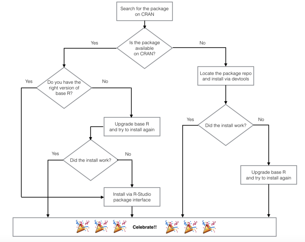
There are a couple common problems that we all encounter when trying to use packages. The most common one is installation issues, usually stemming from version issues (i.e. the version of R doesn’t support the version of a package), and that end up giving frustrating messages like Warning in install.packages : package "magrittr" is not available (for R version 3.3.3). The data blogger Laura Ellis has an excellent flowchart of how to go about installing a package that is worth taking some time to consider.
Let’s walk through this process for another package we’ll use a lot in this R Manual, ggplot2. First, let’s head over to CRAN and go to the list of available packages, sorted by name:
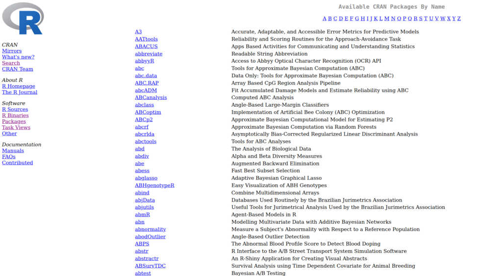
And we can scroll to find the package ggplot2:
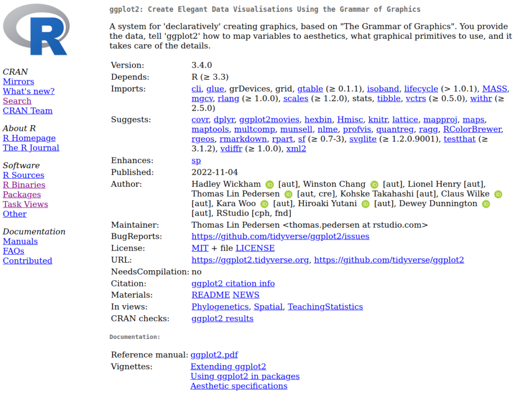
We see here that it Depends: on R (≥ 3.3). We can see what version we’re running by putting the following command in the console:
version## _
## platform x86_64-pc-linux-gnu
## arch x86_64
## os linux-gnu
## system x86_64, linux-gnu
## status Patched
## major 4
## minor 2.2
## year 2022
## month 11
## day 10
## svn rev 83330
## language R
## version.string R version 4.2.2 Patched (2022-11-10 r83330)
## nickname Innocent and TrustingAnd we see here that (at least on this computer), we’re running version 4.2.2, which is ≥ 3.3, so we know we’re okay to download this package. We can do so via the method shown earlier:
install.packages("ggplot2")## Installing package into '//home/user/R/x86_64-pc-linux-gnu-library/4.2'
## (as 'lib' is unspecified)
## also installing the dependencies 'gtable', 'isoband', 'scales', 'tibble', 'withr'
##
## trying URL 'https://cloud.r-project.org/src/contrib/gtable_0.3.3.tar.gz'
## Content type 'application/x-gzip' length 62130 bytes (60 KB)
## downloaded 60KB
## ... (similar output for other dependencies) ...
## trying URL 'https://cloud.r-project.org/src/contrib/ggplot2_3.4.2.tar.gz'
## Content type 'application/x-gzip' length 4013302 bytes (3.8 MB)
## ==================================================
## downloaded 3.8 MB
##
## * installing *source* package 'ggplot2' ...
## ** package 'ggplot2' successfully unpacked and MD5 sums checked
## ** using staged installation
## ** R
## ** inst
## ** byte-compile and prepare package for lazy loading
## ** help
## *** installing help indices
## ** building package indices
## ** testing if installed package can be loaded from temporary location
## ** testing if installed package can be loaded from final location
## ** DONE (ggplot2)
##
## The downloaded source packages are in
## '/tmp/RtmpXXXXXX/downloaded_packages'And we see this worked! On to the next step: Celebrate 🙂
If you receive messages on your computer about specific “dependencies” that you’re missing, the first thing to do is try manually installing the packages the error message is telling you you might need.
Once you have a package loaded in R, it’s usually easy at that point to check out the package functions and find out more about them. For example, since we’ve installed ggplot2, we could load the package, and then use the ? help function to take a look at some of the functions in the package.
library(ggplot2)Now that the package is loaded, let’s take a look at the main function in this package: ggplot()
?ggplotIf you do this in RStudio, the help window on the bottom right will open up a help page that looks something like this:
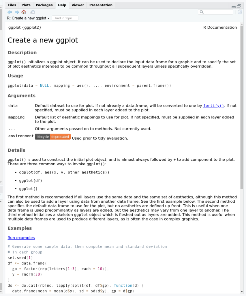
And if you scroll down, you’ll see examples of this function at work. It’s very important to get some sense for how a package/set of functions work before you use them with your own data, else you risk introducing errors that you will be unaware of, simply through unintentional misuse of the function.
Conclusion
Packages are a cornerstone of working effectively in R, extending its capabilities far beyond the base installation. They provide specialized tools for a vast array of tasks, from data manipulation and visualization to complex statistical modeling and bioinformatics analyses.
Throughout this article, you’ve learned how to find, install (from CRAN, Bioconductor, and GitHub), load, and update packages. You’ve also seen the importance of understanding namespaces and using the :: operator to avoid ambiguity when functions from different packages share the same name. While managing packages might seem a bit technical at first, these skills are fundamental to a smooth and reproducible R workflow.