Differential Gene Expression Analysis
Differential gene expression analysis is a fundamental technique in bioinformatics that allows us to identify genes that are differentially expressed between two or more conditions. This article introduces the concept of differential gene expression analysis, with a focus on applications in evolutionary genetics and microbiome studies.
Introduction
In the field of ecology and evolutionary biology, understanding how genes are expressed differently across various conditions, species, or environments is crucial for unraveling the molecular mechanisms underlying adaptation, speciation, and ecological interactions. Differential gene expression analysis provides a powerful framework for identifying these expression changes and their biological significance.
At its core, differential gene expression analysis involves comparing gene expression levels between two or more biologically distinct conditions to identify genes whose expression patterns differ significantly. These differences may arise from various biological phenomena such as:
- Environmental changes (e.g., temperature, pH, nutrient availability)
- Developmental stages (e.g., embryonic, juvenile, adult)
- Disease states (e.g., healthy vs. infected individuals)
- Evolutionary adaptations (e.g., comparing closely related species)
- Experimental treatments (e.g., control vs. drug-treated organisms)
Measuring Gene Expression: RNA Sequencing
RNA sequencing (RNA-seq) is the most common method for measuring gene expression on a genome-wide scale. This technique involves:
- Extracting total RNA from biological samples
- Converting RNA to complementary DNA (cDNA)
- Sequencing the cDNA using high-throughput sequencing technologies
- Mapping the resulting reads to a reference genome or transcriptome
- Counting the number of reads mapped to each gene
The output of an RNA-seq experiment is typically a counts matrix, where rows represent genes, columns represent samples, and each cell contains the number of reads mapped to that gene in that sample. These raw counts serve as the foundation for differential expression analysis.
It’s count data, so can’t we just use a GLM with a poisson distribution?
At first glance, RNA-seq count data might seem like a perfect candidate for a Poisson distribution. After all, counts are discrete, non-negative integers that represent the number of reads mapping to each gene. Recall that the Poisson distribution is commonly used for modeling count data, with its probability mass function given by:
P(X = k) = \frac{\lambda^k e^{-\lambda}}{k!}where \(\lambda\) is both the mean and variance of the distribution. However, RNA-seq data violates a fundamental assumption of the Poisson distribution: the equality of mean and variance.
In RNA-seq experiments, we observe a phenomenon called “overdispersion,” where the variance is consistently larger than the mean. This overdispersion arises from two main sources:
- Technical variation: Differences in sequencing depth, library preparation, and other technical factors
- Biological variation: Even genetically identical organisms raised in the same environment will exhibit some variation in gene expression
When we plot the mean counts against the variance for genes in an RNA-seq dataset, we typically observe a pattern where variance increases more rapidly than the mean, especially for genes with higher expression levels. This relationship is inconsistent with the Poisson distribution, which assumes that variance equals the mean.
The Negative Binomial Distribution: A Better Model for RNA-seq Data
To address the overdispersion in RNA-seq data, the negative binomial distribution provides a more appropriate model. The negative binomial distribution is a discrete probability distribution that models the number of failures in a sequence of independent and identically distributed Bernoulli trials before a specified number of successes occurs.
The probability mass function of the negative binomial distribution is:
\[P(X = k) = \binom{k + r – 1}{k} (1-p)^r p^k\]
where \(r\) is the number of successes, \(p\) is the probability of success in each trial, and \(k\) is the number of failures.
For RNA-seq data analysis, we often parameterize the negative binomial distribution in terms of its mean (\(\mu\)) and dispersion (\(\alpha\)), where:
\[\mu = \frac{r(1-p)}{p}\]
\[\alpha = \frac{1}{r}\]
The variance of the negative binomial distribution is:
\[\sigma^2 = \mu + \alpha\mu^2\]
This formulation allows the variance to be larger than the mean, with the degree of overdispersion controlled by the dispersion parameter \(\alpha\). When \(\alpha\) approaches zero, the negative binomial distribution approaches a Poisson distribution.
The negative binomial distribution is particularly well-suited for RNA-seq data because:
- It can model count data with varying levels of overdispersion
- It allows for different dispersion values for different genes
- It can accommodate the relationship between mean and variance observed in RNA-seq data
The Challenge of Differential Expression Analysis
At first glance, identifying differentially expressed genes might seem straightforward: simply compare the counts between conditions and identify genes with large differences. However, several challenges complicate this analysis:
- Technical variation: Differences in sequencing depth, library preparation, and other technical factors can introduce noise into the data
- Biological variation: Even genetically identical organisms raised in the same environment will exhibit some variation in gene expression
- Count distribution: RNA-seq count data follows a non-normal distribution, making traditional statistical tests inappropriate
- Multiple testing: When analyzing thousands of genes simultaneously, the probability of false positives increases dramatically
To address these challenges, specialized statistical methods have been developed for differential expression analysis. One of the most widely used approaches is implemented in the DESeq2 package for R, which we will explore in detail in this article.
The DESeq2 Approach
DESeq2 is a powerful and widely-used R package for differential expression analysis of RNA-seq data. It addresses the challenges mentioned above through a sophisticated statistical framework that:
- Normalizes data to account for differences in sequencing depth and library composition
- Models count data using a negative binomial distribution, which better captures the variance-mean relationship in RNA-seq data
- Estimates dispersion (variance) parameters for each gene, with sharing of information across genes to improve estimates
- Fits a generalized linear model to test for differential expression
- Applies multiple testing correction to control the false discovery rate
The DESeq2 workflow involves several key steps:
- Size factor estimation: DESeq2 uses the median of ratios method to estimate size factors that normalize for differences in sequencing depth and library composition
- Dispersion estimation: For each gene, DESeq2 estimates a dispersion parameter (\(\alpha\)) that controls the variance-mean relationship in the negative binomial model
- Model fitting: DESeq2 fits a generalized linear model for each gene, with the design formula specifying the experimental design
- Statistical testing: DESeq2 uses a Wald test to determine whether the estimated coefficients are significantly different from zero
- Multiple testing correction: DESeq2 applies the Benjamini-Hochberg procedure to control the false discovery rate
The result of a DESeq2 analysis is a list of genes that are significantly differentially expressed between conditions, along with estimates of their fold changes and adjusted p-values.
The LETS1 Dataset: An Example Case Study
To demonstrate differential gene expression analysis in practice, we will work with a dataset from a study on long non-coding RNA (lncRNA) in cancer research. This dataset examines the effects of a tumor-promoting lncRNA called LETS1 (lncRNA enabling TGF-beta signaling 1).
Previous research with this lncRNA found that LETS1 potentiates epithelial-to-mesenchymal transition (EMT), a critical process in cancer progression that allows epithelial cells to gain migratory and invasive properties. LETS1 was also shown to enhance cell migration and extravasation (the movement of cells out of circulation and into tissues) in a zebrafish xenograft model.
To better understand the molecular mechanisms through which LETS1 exerts these effects, the researchers designed an experiment with the following characteristics:
- Experimental design: LETS1 was overexpressed in A549 cells (a human lung adenocarcinoma cell line) using a lentiviral vector. Control cells were transduced with an empty vector (Co.vec).
- Treatment conditions: Some cells were treated with TGF-beta, a growth factor known to induce EMT, while others were left untreated as controls.
- Replication: Three biological replicates were included for each combination of LETS1 expression and TGF-beta treatment.
Throughout this article, we will use this dataset to illustrate the key steps in differential expression analysis, from data preprocessing to interpretation of results.
Obtaining and Processing RNA-seq Data
The first step in any differential expression analysis is to obtain the count data and prepare it for analysis. In this section, we’ll walk through the process of downloading RNA-seq count data from a public repository, creating the necessary metadata, and preparing it for analysis with DESeq2.
Downloading Count Data from NCBI GEO
The National Center for Biotechnology Information (NCBI) Gene Expression Omnibus (GEO) is a public repository for high-throughput gene expression data.
For our analysis, we’ll download the count data for the LETS1 study from GEO.
library(tidyverse)

# Prepare the URLs for the counts and annotation files
url_base <- "https://www.ncbi.nlm.nih.gov/geo/download/?format=file&type=rnaseq_counts"
url_counts <- paste0(url_base, "&acc=GSE203159&file=GSE203159_raw_counts_GRCh38.p13_NCBI.tsv.gz")
url_annot <- paste0(url_base, "&file=Human.GRCh38.p13.annot.tsv.gz")

# Load counts table
tbl_counts <- data.table::fread(url_counts, header = TRUE, colClasses = "integer", data.table = FALSE)

# Set the row names to the GeneID column and pop it off
rownames(tbl_counts) <- tbl_counts$GeneID
tbl_counts <- tbl_counts[, -1] # remove the GeneID column

tbl_counts %>%
  as_tibble()
# A tibble: 24,053 × 12
GSM6160812 GSM6160813 GSM6160814 GSM6160815 GSM6160816 GSM6160817 GSM6160818 GSM6160819 GSM6160820 GSM6160821 GSM6160822 GSM6160823
1 8 11 9 10 9 7 8 8 9 10 6 6
2 329 377 345 331 366 337 361 387 328 350 324 317
3 5 7 2 5 6 8 4 4 8 6 6 7
4 54 53 53 36 39 43 50 61 62 33 39 32
5 54 62 54 49 40 44 43 52 33 36 41 34
6 18 22 25 18 15 12 13 26 20 18 14 19
7 397 404 403 365 450 385 381 423 396 374 397 359
8 4 2 3 4 7 4 4 3 6 4 4 5
9 4 9 6 5 6 6 5 8 4 6 7 3
10 91 88 72 76 66 73 73 95 70 62 74 51
# ℹ 24,043 more rows Pre-filtering the Count Data
Before proceeding with the analysis, it’s common to pre-filter the count data to remove genes with very low expression, which are unlikely to be informative. This step helps reduce the computational burden and can improve the statistical power of the analysis.
<pre class="wp-block-eeb-code-block"><code class="language-r"># Pre-filter the counts table to keep only genes with at least 10 counts across all samples
mask_keep <- rowSums(tbl_counts) >= 10
tbl_counts <- tbl_counts[mask_keep, ]</code></pre>
Getting the Annotations
We can retrieve the annotations. Since there are numerous unneeded columns, we will restrict ourselves to the most pertinent ones: gene ID, gene symbol, and a description of the gene for our own reference.
annot <- data.table::fread(url_annot, header = TRUE, quote = "", stringsAsFactors = FALSE, data.table = FALSE) %>%
  as_tibble() %>%
  select(GeneID, Symbol, Description) %>%
  # Keep only the rows that are present in the counts table
  filter(GeneID %in% rownames(tbl_counts))
annot
# A tibble: 24,053 × 3
GeneID Symbol Description
1 100287102 DDX11L1 DEAD/H-box helicase 11 like 1 (pseudogene)
2 653635 WASH7P WASP family homolog 7, pseudogene
3 102466751 MIR6859-1 microRNA 6859-1
4 100996442 LOC100996442 WAS protein family homolog 2-like
5 729737 LOC729737 uncharacterized LOC729737
6 102725121 DDX11L17 DEAD/H-box helicase 11 like 17 (pseudogene)
7 102723897 WASH9P WAS protein family homolog 9, pseudogene
8 102465909 MIR6859-2 microRNA 6859-2
9 112268260 LOC112268260 uncharacterized LOC112268260
10 100132287 LOC100132287 uncharacterized LOC100132287
# ℹ 24,043 more rows Creating the Sample Metadata
For DESeq2 to understand the experimental design, we need to create a metadata table (also called a sample information or colData table) that describes the experimental factors associated with each sample. In our case, we have two factors: genotype (control or LETS1Overexpressed) and treatment (control or TGFB).
df_meta <- data.frame(
  genotype_grp = rep(c("control", "LETS1Overexpressed"), each = 6) %>% fct_relevel("control"),
  treatment_grp = rep(c("control", "TGFB"), each = 3, times = 2) %>% fct_relevel("control")
)
# The rownames of this table should be the same as the column names of the counts table
rownames(df_meta) <- colnames(tbl_counts)
df_meta
genotype_grp treatment_grp
GSM6160812 control control
GSM6160813 control control
GSM6160814 control control
GSM6160815 control TGFB
GSM6160816 control TGFB
GSM6160817 control TGFB
GSM6160818 LETS1Overexpressed control
GSM6160819 LETS1Overexpressed control
GSM6160820 LETS1Overexpressed control
GSM6160821 LETS1Overexpressed TGFB
GSM6160822 LETS1Overexpressed TGFB
GSM6160823 LETS1Overexpressed TGFBCreating the DESeqDataSet Object
With our count data and metadata prepared, we can now create a DESeqDataSet object, which is the central data structure used by DESeq2.
ds_dataset <- DESeq2::DESeqDataSetFromMatrix(
  countData = tbl_counts, # the count matrix
  colData = df_meta, # the metadata table
  design = ~ genotype_grp * treatment_grp # the design formula
)
The DESeqDataSetFromMatrix function takes three main arguments:
- countData: The count matrix, with genes in rows and samples in columns
- colData: The metadata table, with samples in rows and experimental factors in columns
- design: A formula specifying the experimental design
In our case, the design formula is ~ genotype_grp * treatment_grp, which indicates that we want to model the effects of both genotype_grp and treatment_grp, as well as their interaction. This formula expands to ~ genotype_grp + treatment_grp + genotype_grp:treatment_grp, where the last term represents the interaction between the two factors.
Exploring the Data with Principal Component Analysis (PCA)
Before proceeding with the differential expression analysis, it’s a good practice to explore the data to identify patterns and potential issues. Principal Component Analysis (PCA) is a dimensionality reduction technique that can help visualize the relationships between samples in a dataset.
PCA works by identifying the directions (principal components) along which the variance in the data is maximized. By projecting the data onto these principal components, we can visualize the major sources of variation in a lower-dimensional space, typically a 2D plot.
In the context of RNA-seq data, PCA can help us:
- Identify sample outliers that might need to be removed or handled specially
- Verify that samples cluster according to the experimental factors of interest
- Identify unexpected sources of variation, such as batch effects
- Assess the relative importance of different experimental factors in explaining the overall variation in the data
DESeq2::vst(ds_dataset) %>%
  DESeq2::plotPCA(intgroup = c("genotype_grp", "treatment_grp")) +
  labs(title = "PCA Plot", color = "Group") +
  ggthemes::theme_base()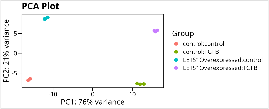
This PCA plot allows us to visualize the overall patterns in our data. If the experimental factors are indeed the major sources of variation, we would expect to see clear separation between the experimental groups. In our case, we indeed see excellent separation between the experimental groups. This confirms that our experimental design is capturing the major sources of variation in the data
Fitting the Model
After creating our DESeqDataSet object and exploring the data with PCA, we are ready to run the differential expression analysis by fitting a negative binomial model to the count data. The core function DESeq() performs several important steps:
- Size factor estimation: Normalizes for differences in sequencing depth between samples
- Dispersion estimation: Estimates the dispersion parameter for each gene that controls the variance
- Model fitting: Fits a negative binomial generalized linear model for each gene based on the design formula
- Hypothesis testing: Tests for differential expression using the Wald test
# Run the DESeq2 model
ds_model <- DESeq2::DESeq(ds_dataset, test = "Wald", sfType = "poscount")
estimating size factors
estimating dispersions
gene-wise dispersion estimates
mean-dispersion relationship
final dispersion estimates
fitting model and testingThe output shows that DESeq2 proceeds through each of these steps automatically. The test = "Wald" parameter specifies that we want to use the Wald test for significance testing, which is efficient for testing individual model coefficients. The sfType = "poscount" parameter indicates that we want to use the “positive counts” method for estimating size factors, which is suitable for our dataset.
Once we have fitted our model, we can see which coefficients (contrasts) are available for testing by using the resultsNames() function:
# Check available result names
DESeq2::resultsNames(ds_model)
[1] "Intercept" "genotype_grp_LETS1Overexpressed_vs_control" "treatment_grp_TGFB_vs_control" "genotype_grpLETS1Overexpressed.treatment_grpTGFB"These result names correspond to the terms in our model:
- “Intercept” represents the reference level (control genotype with control treatment)
- “genotype_grp_LETS1Overexpressed_vs_control” represents the effect of LETS1 overexpression
- “treatment_grp_TGFB_vs_control” represents the effect of TGFB treatment
- “genotype_grpLETS1Overexpressed.treatment_grpTGFB” represents the interaction between LETS1 overexpression and TGFB treatment
Contrasts – Basic Contrast
To extract results from the model, we use the results() function with a specified contrast. A contrast defines the comparison we want to make between different experimental conditions. DESeq2 offers flexible ways to specify contrasts, depending on the biological question we’re addressing.
Let’s start with a simple contrast: comparing gene expression between control and LETS1-overexpressed cells, averaged across both treatment conditions (control and TGFB). This allows us to identify genes affected by LETS1 overexpression regardless of TGFB treatment.
# The contrast below compares the control vs LETS1Overexpressed genotypes, but averaged across the 2 treatment groups
res_ctrl_vs_LETS1 <- DESeq2::results(
  ds_model,
  contrast = c("genotype_grp", "control", "LETS1Overexpressed"),
  alpha = 0.05,
  pAdjustMethod = "fdr"
) %>%
  as_tibble() %>%
  # Order is preserved in the results table,
  # so we can immediately join it with the annotation table
  bind_cols(annot)
res_ctrl_vs_LETS1
# A tibble: 24,053 × 9
baseMean log2FoldChange lfcSE stat pvalue padj GeneID Symbol Description
1 8.42 0.184 0.605 0.304 0.761 0.914 100287102 DDX11L1 DEAD/H-box helicase 11 like 1 (pseudogene)
2 346. -0.0135 0.107 -0.126 0.900 0.967 653635 WASH7P WASP family homolog 7, pseudogene
3 5.68 -0.173 0.782 -0.221 0.825 NA 102466751 MIR6859-1 microRNA 6859-1
4 46.1 -0.0924 0.254 -0.363 0.716 0.896 100996442 LOC100996442 WAS protein family homolog 2-like
5 45.1 0.430 0.271 1.59 0.112 0.359 729737 LOC729737 uncharacterized LOC729737
6 18.3 0.160 0.424 0.377 0.706 0.892 102725121 DDX11L17 DEAD/H-box helicase 11 like 17 (pseudogene)
7 394. 0.0252 0.102 0.248 0.804 0.932 102723897 WASH9P WAS protein family homolog 9, pseudogene
8 4.18 -0.510 0.899 -0.567 0.571 NA 102465909 MIR6859-2 microRNA 6859-2
9 5.75 0.180 0.747 0.242 0.809 NA 112268260 LOC112268260 uncharacterized LOC112268260
10 74.1 0.0965 0.220 0.439 0.661 0.872 100132287 LOC100132287 uncharacterized LOC100132287
# ℹ 24,043 more rows The results table contains several important columns:
- baseMean: The average normalized count across all samples
- log2FoldChange: The log2 fold change between conditions (positive values indicate higher expression in LETS1-overexpressed cells)
- lfcSE: The standard error of the log2 fold change estimate
- stat: The Wald statistic (log2FoldChange / lfcSE)
- pvalue: The raw p-value from the Wald test
- padj: The p-value adjusted for multiple testing using the FDR method
- GeneID, Symbol, Description: Information from the annotation table
Genes with a low adjusted p-value (padj) are considered significantly differentially expressed. The log2FoldChange indicates the direction and magnitude of the expression change.
Contrasts – Fine-tuned Selection
Sometimes we need to make more complex comparisons that involve multiple factors and their interactions. For example, we might want to compare the control cells under control conditions with LETS1-overexpressed cells under TGFB treatment, which involves both main effects and their interaction.
DESeq2 allows us to combine multiple terms from the model to create custom contrasts. This is especially useful for factorial designs like ours, where we have multiple factors (genotype and treatment) and are interested in specific combinations of factor levels.
# For comparing controls_controls vs LETS1Overexpressed_TGFB, we need to combine the main effects and interaction
res_ctrl_vs_LETS1_TGFB <- DESeq2::results(
  ds_model,
  # The contrast combines the LETS1Overexpressed effect, TGFB effect, and their interaction
  contrast = list(
    c(
      "genotype_grp_LETS1Overexpressed_vs_control",
      "treatment_grp_TGFB_vs_control",
      "genotype_grpLETS1Overexpressed.treatment_grpTGFB"
    ),
    character()
  ),
  alpha = 0.001,
  pAdjustMethod = "fdr"
) %>%
  as_tibble() %>%
  bind_cols(annot)
# This contrast specification works because:
# The numerator (first element of the list) combines all the terms needed to go from control_control to LETS1Overexpressed_TGFB:
# The main effect of LETS1Overexpressed vs control
# The main effect of TGFB vs control
# The interaction term that accounts for the non-additive effects
# The denominator (second element) is empty, meaning we're comparing against the baseline
# This will give you the specific comparison you're looking for between control samples under control conditions versus LETS1Overexpressed samples under TGFB treatment.
res_ctrl_vs_LETS1_TGFB
# A tibble: 24,053 × 9
baseMean log2FoldChange lfcSE stat pvalue padj GeneID Symbol Description
1 8.42 -0.303 0.614 -0.493 0.622 0.747 100287102 DDX11L1 DEAD/H-box helicase 11 like 1 (pseudogene)
2 346. -0.0407 0.108 -0.377 0.706 0.810 653635 WASH7P WASP family homolog 7, pseudogene
3 5.68 0.486 0.769 0.631 0.528 0.669 102466751 MIR6859-1 microRNA 6859-1
4 46.1 -0.578 0.270 -2.15 0.0319 0.0752 100996442 LOC100996442 WAS protein family homolog 2-like
5 45.1 -0.571 0.275 -2.08 0.0378 0.0866 729737 LOC729737 uncharacterized LOC729737
6 18.3 -0.306 0.430 -0.711 0.477 0.625 102725121 DDX11L17 DEAD/H-box helicase 11 like 17 (pseudogene)
7 394. -0.0479 0.102 -0.469 0.639 0.761 102723897 WASH9P WAS protein family homolog 9, pseudogene
8 4.18 0.575 0.899 0.639 0.523 NA 102465909 MIR6859-2 microRNA 6859-2
9 5.75 -0.205 0.752 -0.273 0.785 0.866 112268260 LOC112268260 uncharacterized LOC112268260
10 74.1 -0.381 0.225 -1.69 0.0905 0.177 100132287 LOC100132287 uncharacterized LOC100132287
# ℹ 24,043 more rows This complex contrast allows us to identify genes that are differentially expressed when both LETS1 is overexpressed and TGFB is present, compared to the baseline condition (control genotype with control treatment). This is particularly relevant to our biological question, as we want to understand how LETS1 affects gene expression in the context of TGF-beta signaling.
With our results in hand, we can now visualize the differential expression patterns to gain insights into the biological processes affected by LETS1 and TGF-beta. Visualization is a crucial step in differential expression analysis, as it allows us to identify patterns and select candidate genes for further investigation.
Visualizing Differential Gene Expression
Dispersion Plot
The dispersion plot is a diagnostic tool that shows the relationship between the mean expression level and the estimated dispersion for each gene. It helps us assess how well the negative binomial model fits our data and whether the dispersion estimation process was effective.
In this plot:
- Each black dot represents a gene with its estimated dispersion based on that gene alone
- The red curve represents the fitted relationship between mean expression and dispersion
- The blue dots represent the final dispersion estimates used in the model, which incorporate information from the fitted trend
A good dispersion plot should show a clear trend where dispersion decreases as mean expression increases, with most genes following this trend and relatively few outliers.
DESeq2::plotDispEsts(
  ds_model,
  main = "Dispersion Estimates",
  xlab = "Mean of Normalized Counts",
  ylab = "Dispersion"
)
Our dispersion plot shows the expected trend of decreasing dispersion with increasing mean expression. The blue dots (final dispersion estimates) generally follow the red trend line, indicating that the dispersion estimation process worked well. Some genes have higher dispersion values (above the trend), which is typical for RNA-seq data and reflects biological variability that the model will account for. The plot confirms that our negative binomial model with estimated dispersions is appropriate for this dataset.
Volcano Plot
A volcano plot is one of the most informative visualizations for differential expression analysis. It plots the statistical significance (-log10 of the adjusted p-value) against the magnitude of change (log2 fold change) for each gene, allowing us to quickly identify genes that show both large and statistically significant expression changes.
In a volcano plot:
- Genes in the upper right are significantly upregulated (high positive log2 fold change and low p-value)
- Genes in the upper left are significantly downregulated (high negative log2 fold change and low p-value)
- Genes near the bottom are not significantly differentially expressed
# Thresholds for color-coding the points in the volcano plot
thres_fold_change <- 1
thres_padj <- 0.05

# Thresholds for annotation of exceptional points in the volcano plot
candidate_thres_fold_change <- 2
candidate_thres_padj <- 1E-100

volcano_data <- res_ctrl_vs_LETS1_TGFB %>%
  mutate(
    significant = padj < thres_padj & abs(log2FoldChange) >= thres_fold_change,
    sig_text = padj < candidate_thres_padj & abs(log2FoldChange) >= candidate_thres_fold_change,
    direction = case_when(
      significant & log2FoldChange > 0 ~ "Up",
      significant & log2FoldChange < 0 ~ "Down",
      TRUE ~ "Not Significant"
    ),
    symbol = case_when(
      sig_text & log2FoldChange > 0 ~ paste0("<span style='color: #FF3030;'>", Symbol, "</span>"),
      sig_text & log2FoldChange < 0 ~ paste0("<span style='color: #00BFFF;'>", Symbol, "</span>"),
      TRUE ~ NA_character_
    )
  )

volcano_plot <- ggplot(volcano_data, aes(x = log2FoldChange, y = -log10(padj), label = symbol)) +
  geom_point(aes(color = direction), alpha = 0.6) +
  scale_color_manual(values = c("Down" = "#00BFFF", "Up" = "#FF3030", "Not Significant" = "grey")) +
  geom_hline(yintercept = -log10(thres_padj), linetype = "dashed", color = "grey50") +
  geom_vline(xintercept = c(-thres_fold_change, thres_fold_change), linetype = "dashed", color = "grey50") +
  ggtext::geom_richtext(aes(label = symbol), size = 3, color = "black") +
  labs(
    title = "Volcano Plot: Control vs LETS1Overexpressed with TGFB",
    x = "log2 Fold Change",
    y = "-log10(adjusted p-value)",
    color = "Direction"
  ) +
  ggthemes::theme_base() +
  theme(legend.position = "bottom")
volcano_plot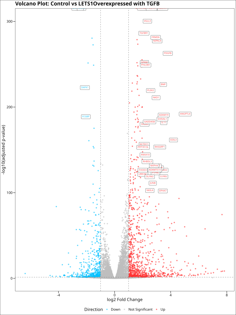
Our volcano plot shows a classic “volcano” shape, with many genes significantly differentially expressed between control cells under control conditions and LETS1-overexpressed cells under TGFB treatment. The genes are color-coded based on the direction of change (upregulated in red, downregulated in blue), and the horizontal and vertical dashed lines represent our significance thresholds.
The genes that show the most dramatic and significant changes are prime candidates for follow-up studies. These might include:
- Functional validation studies to confirm their role in LETS1 and TGF-beta signaling
- Pathway enrichment analysis to identify biological processes affected by LETS1 and TGF-beta
- Literature reviews to connect these genes to known functions in epithelial-to-mesenchymal transition (EMT)
- Protein-protein interaction studies to understand how these genes might interact with LETS1 or components of the TGF-beta pathway
MA Plot
An MA plot (Mean-Average plot) is another useful visualization for differential expression analysis. It plots the log2 fold change (M) against the mean of normalized counts (A) for each gene. This allows us to assess whether there’s any relationship between expression level and fold change, which could indicate biases in the analysis.
In an ideal MA plot:
- The majority of points should be centered around the y = 0 line (no change in expression)
- The spread of points should be relatively even across the x-axis (no bias by expression level)
- Only a minority of points should be significantly differentially expressed (colored points)
ma_plot <- ggplot(volcano_data, aes(x = log10(baseMean), y = log2FoldChange)) +
  geom_point(aes(color = direction), alpha = 0.6) +
  scale_color_manual(values = c("Down" = "#00BFFF", "Up" = "#FF3030", "Not Significant" = "grey")) +
  geom_hline(yintercept = 0, linetype = "dashed", color = "grey50") +
  labs(
    title = "MA Plot: Control vs LETS1Overexpressed with TGFB",
    x = "log10(mean of normalized counts)",
    y = "log2 Fold Change",
    color = "Direction"
  ) +
  theme(legend.position = "bottom") +
  ggthemes::theme_base()
ma_plot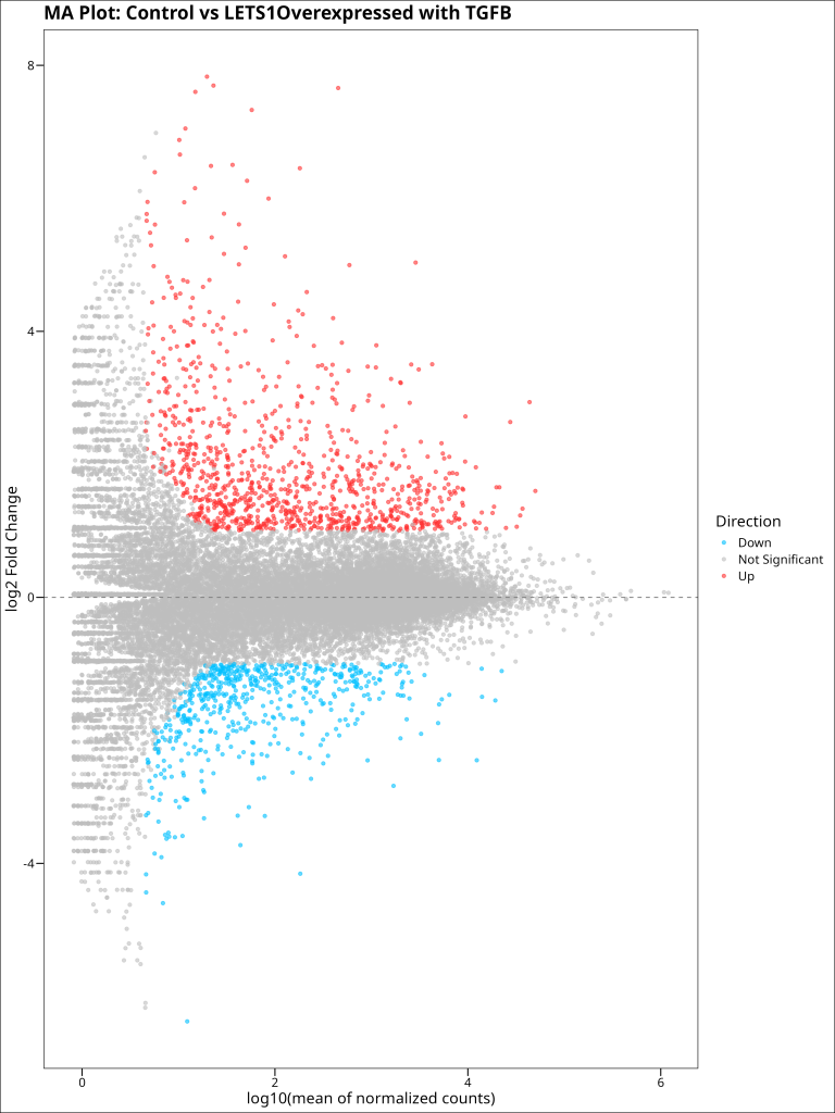
Our MA plot shows several important patterns:
- The majority of genes (gray points) are centered around the y = 0 line, indicating no differential expression
- Significantly differentially expressed genes (colored points) are distributed across the range of expression levels, with no obvious bias
- The spread of points narrows at lower expression levels, which is expected due to the higher variance of low-count genes
- Some genes show very large fold changes (far from y = 0), particularly among the moderately to highly expressed genes
This plot confirms that our differential expression analysis is technically sound, with no major biases affecting the results. It also highlights that genes across a range of expression levels are affected by LETS1 overexpression and TGFB treatment, suggesting a broad impact on the transcriptome.
Summary
In this article, we’ve explored the principles and practice of differential gene expression analysis using RNA-seq data. We’ve covered the complete workflow from data acquisition to visualization.
Key points from our analysis include:
- The importance of using an appropriate statistical model (negative binomial) for RNA-seq count data
- The process of creating a DESeqDataSet and fitting a model that accounts for experimental design factors
- The use of contrasts to test specific biological hypotheses about gene expression differences
- The value of data visualization in interpreting and validating differential expression results
As with any computational analysis, it’s important to remember that statistical significance doesn’t necessarily imply biological significance. The genes identified as differentially expressed should be interpreted in the context of prior knowledge and validated through additional experiments before drawing firm conclusions about their functional roles.
Overall, differential gene expression analysis is a powerful tool for exploring the molecular basis of biological phenomena, and the DESeq2 package provides a robust and flexible framework for conducting these analyses in R.