Setting Up Your R Environment

To work with phylogenetic trees in R, we’ll need several specialized packages. Here’s how to install and load them:

# Install required packages if you haven't already
install.packages(c("tidyverse", "ape"))
if (!requireNamespace("BiocManager", quietly = TRUE))
    install.packages("BiocManager")
BiocManager::install("ggtree")

# Load the packages
library(tidyverse)
library(ape)      # For tree manipulation and basic plotting
library(ggtree)   # For advanced and customizable tree plotting
library(phytools) # For additional tree utilities

Tree Objects

In R, phylogenetic trees can be represented in several different formats. The most common is the phylo object from the ape package, which is the standard format for phylogenetic trees in R. You can obtain tree objects in several ways:

• Built-in datasets: Many packages come with example trees (like bird.orders in ape)
• Tree files: Import trees from Newick or Nexus files using ape::read.tree() or ape::read.nexus()
• Tree building: Construct trees from sequence data using methods like Neighbor-Joining or Maximum Likelihood
• Tree manipulation: Create new trees by modifying existing ones (e.g., pruning tips, re-rooting)

Pre-built Trees: The Bird Orders Example

Let’s start by examining a pre-built phylogenetic tree of bird orders that comes with the ape package. This tree represents the evolutionary relationships between different orders of birds.

# Load the bird.orders data
data(bird.orders)

# Examine the structure of the tree
str(bird.orders)

List of 4
 $ edge       : int [1:44, 1:2] 24 25 26 26 25 27 28 28 27 24 ...
 $ Nnode      : int 22
 $ tip.label  : chr [1:23] "Struthioniformes" "Tinamiformes" "Craciformes" "Galliformes" ...
 $ edge.length: num [1:44] 2.1 4.1 21.8 21.8 3 1.3 21.6 21.6 22.9 1 ...
 - attr(*, "class")= chr "phylo"

The output shows us that bird.orders is a phylo object, which is R’s standard format for phylogenetic trees. Let’s break down its components:

• edge: A matrix showing how nodes are connected. Each row represents a branch, with the first column showing the parent node and the second column showing the child node.
• Nnode: The number of internal nodes (22 in this case).
• tip.label: The names of the terminal nodes (23 bird orders).
• edge.length: The lengths of the branches, representing evolutionary distances.

Building Trees from DNA Sequences: The Woodmouse Example

Now, let’s explore how to build a phylogenetic tree from DNA sequence data using the woodmouse dataset. This dataset contains DNA sequences from different woodmouse populations, which we’ll use to infer their evolutionary relationships.

# Load the woodmouse data
data(woodmouse)

# Examine the structure of the DNA sequences
str(woodmouse)

 'DNAbin' raw [1:15, 1:965] n a a a ...
 - attr(*, "dimnames")=List of 2
  ..$ : chr [1:15] "No305" "No304" "No306" "No0906S" ...
  ..$ : NULL

The woodmouse data is stored as a DNAbin object, which is a special format for DNA sequence data in R. It contains 15 sequences (representing different woodmouse populations) with 965 base pairs each.

Step 1: Calculating Genetic Distances

To build a phylogenetic tree, we first need to calculate the genetic distances between all pairs of sequences

DNA Evolution Models

When calculating genetic distances, it’s important to choose an appropriate model of DNA evolution. Different models make different assumptions about how DNA sequences change over time. Here are some common models and when to use them.

For our woodmouse example, we’re using the K80 model because it provides a good balance between accuracy and computational efficiency. The woodmouse sequences are moderately divergent, and we want to account for the fact that transitions are more common than transversions in mitochondrial DNA.

# Calculate distance matrix using the K80 model
dist_matrix_woodmouse <- ape::dist.dna(woodmouse, model = "K80")
as.matrix(dist_matrix_woodmouse)[1:5, 1:5]

             No305      No304       No306     No0906S     No0908S
No305   0.00000000 0.01449377 0.013363824 0.017879906 0.016761346
No304   0.01449377 0.00000000 0.003307620 0.012223737 0.011111568
No306   0.01336382 0.00330762 0.000000000 0.008860496 0.007752093
No0906S 0.01787991 0.01222374 0.008860496 0.000000000 0.012223737
No0908S 0.01676135 0.01111157 0.007752093 0.012223737 0.000000000

The distance matrix shows the genetic distances between different woodmouse populations. For example:

• The distance between No305 and No304 is about 0.014, indicating they are relatively distantly related
• No304 and No306 are more closely related, with a distance of only 0.003
• The diagonal values are all 0, as they represent the distance between a sequence and itself

Step 2: Building the Tree

We’ll use the Neighbor-Joining (NJ) method to build our tree. This method is particularly useful because it:

• Doesn’t assume a molecular clock (equal rates of evolution)
• Is computationally efficient
• Works well with distance-based data

# Build a tree using Neighbor-Joining method
woodmouse_tree_nj <- ape::nj(dist_matrix_woodmouse)

We use midpoint rooting (via phytools::midpoint.root()) to place the root of the tree at the midpoint of the longest path between any two tips. This is a common approach when we don’t have a known outgroup.

# Root the tree using midpoint rooting
woodmouse_tree_nj_rooted <- phytools::midpoint.root(woodmouse_tree_nj)
woodmouse_tree_nj_rooted

Phylogenetic tree with 15 tips and 14 internal nodes.

Tip labels:
  No305, No304, No306, No0906S, No0908S, No0909S, ...

Rooted; includes branch length(s).

We use midpoint rooting to place the root of the tree at the midpoint of the longest path between any two tips. This is a common approach when we don’t have a known outgroup.

Tree Visualization

Visualizing phylogenetic trees is crucial for understanding and communicating evolutionary relationships. R offers two main approaches to tree visualization: the basic plotting system in ape and the more sophisticated ggtree package. While ape provides essential functionality for quick visualizations, ggtree offers extensive customization options and modern aesthetics. In this section, we’ll explore both approaches and learn when to use each one.

Basic Plotting with ape

The ape package provides the fundamental plot.phylo() function for visualizing phylogenetic trees. This function is the workhorse of basic tree visualization in R and offers several key features:

• Multiple tree types (phylogram, cladogram, unrooted, etc.)
• Basic customization of branch colors, widths, and tip labels
• Support for both rooted and unrooted trees
• Ability to show or hide branch lengths

ape::plot.phylo(
  bird.orders,
  type = "phylogram", # Default type
  use.edge.length = TRUE, # Use branch lengths (default)
  show.tip.label = TRUE, # Show tip labels (default)
  cex = 0.8, # Tip label size
  font = 3, # Font style for tip labels (e.g., italic)
  edge.color = "blue", # Branch color
  edge.width = 2, # Branch width
  main = "Customized Bird Orders - ape plot"
)

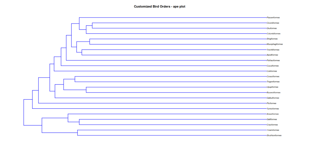
While ape::plot.phylo() is excellent for basic tree visualization, it has some limitations:

• Limited customization options compared to modern plotting systems
• No built-in support for complex annotations or highlighting
• Less flexible layout options
• More challenging to create publication-quality figures

These limitations led to the development of ggtree, which builds on the powerful ggplot2 system to provide more sophisticated tree visualization capabilities.

Plotting with ggtree

The ggtree package extends ggplot2 to handle phylogenetic trees. The main ggtree() function can accept various types of input:

• phylo objects (from ape)
• treedata objects (from treeio)
• phylo4 objects (from phylobase)
• Newick or Nexus tree files

ggtree(woodmouse_tree_nj_rooted) +
  # Add tip labels
  geom_tiplab(
    align = TRUE, # Align labels to the tips
    linesize = 0.5, # Size of connecting line
    linetype = "dotted", # Line type
    size = 3, # Font size
    color = "purple" # Color of the labels
  ) +
  # Add scale bar
  geom_treescale(
    x = 0, y = 14, # Position of scale bar
    fontsize = 3, linesize = 0.5, color = "blue"
  ) +
  labs(title = "Plotting the Woodmouse Phylogenetic Tree with ggtree") +
  theme_tree2() + # Use ggtree's tree-specific theme
  # Add padding to prevent label cutoff
  xlim(NA, max(fortify(woodmouse_tree_nj_rooted)$x) * 1.1) +
  theme(plot.margin = margin(1, 2, 1, 1, "cm"))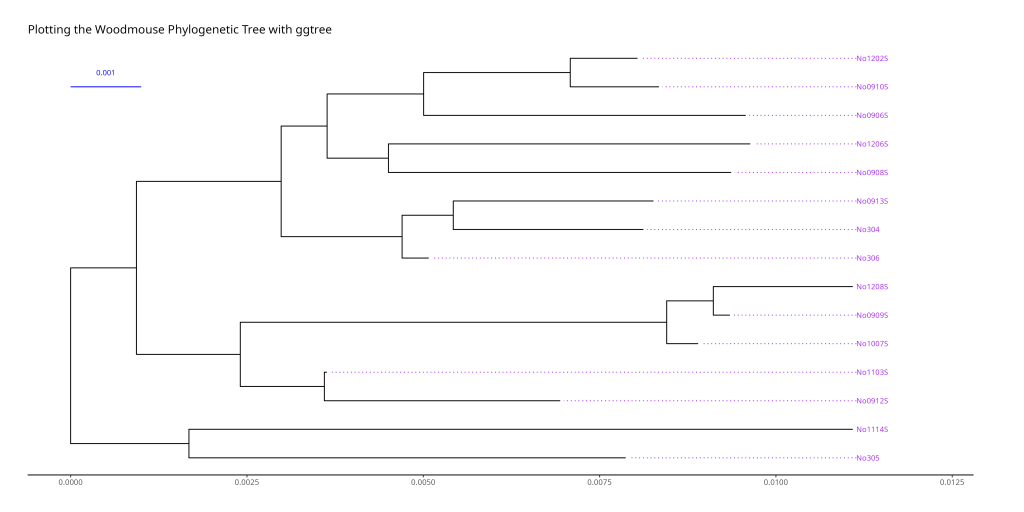

The woodmouse tree figure above demonstrates the power of ggtree’s customization options. The purple tip labels are aligned and connected to the tree with dotted lines, making it easy to read the population names. The blue scale bar in the top-left corner shows the genetic distance scale, helping readers understand the evolutionary distances between populations.

Tree Layouts

ggtree offers several different layouts for visualizing your phylogenetic tree, each with its own advantages:

# Rectangular layout (default)
ggtree::ggtree(bird.orders, layout = "rectangular") +
  ggtree::geom_tiplab(align = TRUE) +
  labs(title = "Layout: Rectangular") +
  ggtree::theme_tree2() +
  # Padding to the right to avoid cutting off the labels
  xlim(NA, max(fortify(bird.orders)$x) * 1.1)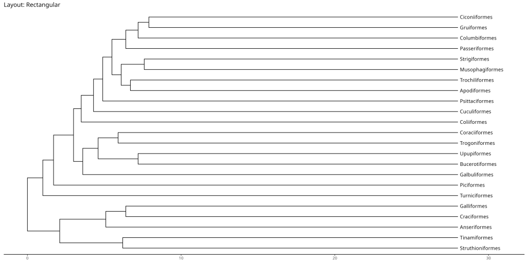

# Slanted layout
ggtree::ggtree(bird.orders, layout = "slanted") +
  ggtree::geom_tiplab(align = TRUE) +
  labs(title = "Layout: Slanted") +
  ggtree::theme_tree2() +
  # Padding to the right to avoid cutting off the labels
  xlim(NA, max(fortify(bird.orders)$x) * 1.1)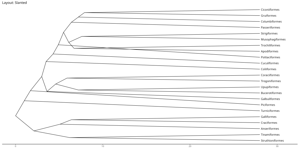

# Circular layout
ggtree::ggtree(bird.orders, layout = "circular") +
  ggtree::geom_tiplab() +
  labs(title = "Layout: Circular") +
  ggtree::theme_tree2() +
  # Padding to the right to avoid cutting off the labels
  xlim(NA, max(fortify(bird.orders)$x) * 1.1)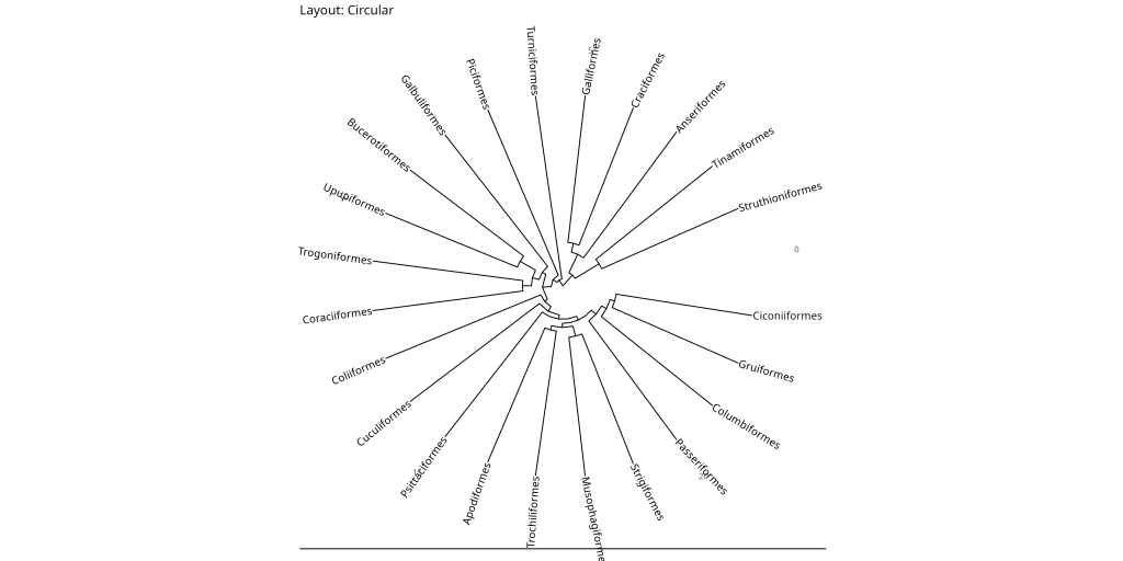

# Fan layout
ggtree::ggtree(bird.orders, layout = "fan", open.angle = 10) +
  ggtree::geom_tiplab() +
  labs(title = "Layout: Fan") + # open.angle to avoid overlap
  ggtree::theme_tree2() +
  # Padding to the right to avoid cutting off the labels
  xlim(NA, max(fortify(bird.orders)$x) * 1.1)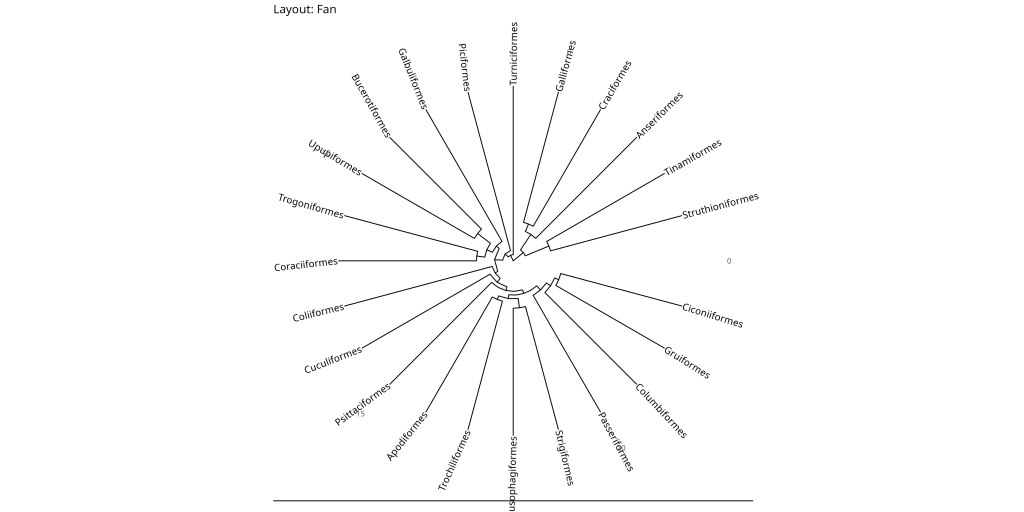

While the fan and circular layouts may appear similar, they serve different purposes. The circular layout maintains equal angles between branches, making it ideal for showing evolutionary relationships in a balanced way. The fan layout, on the other hand, allows for an open angle (controlled by the open.angle parameter), which can help prevent label overlap in dense trees and create more space for annotations.

# Unrooted layout
ggtree::ggtree(woodmouse_tree_nj, layout = "equal_angle") +
  ggtree::geom_tiplab(size = 3) +
  labs(title = "Woodmouse NJ Tree - Unrooted (ggtree)") +
  ggtree::theme_tree2() +
  # Padding to the right to avoid cutting off the labels
  xlim(NA, max(fortify(woodmouse_tree_nj)$x) * 1.1)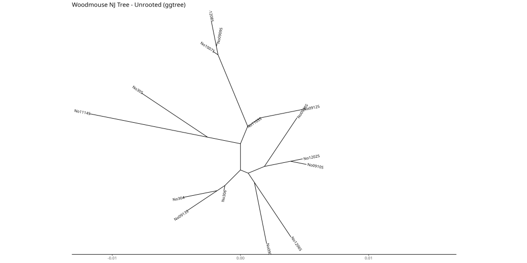

Each layout has specific use cases:

• Rectangular: Best for most purposes, especially when showing evolutionary time
• Slanted: Useful when you want to emphasize the hierarchical structure of the tree while maintaining a compact layout. The slanted lines help distinguish between different levels of the hierarchy more clearly than the rectangular layout.
• Circular: Useful for showing relationships in a compact format
• Fan: Good for large trees where you want to avoid label overlap
• Unrooted: Best when you want to show relationships without assuming a root

Highlighting Clades

A clade is a group of organisms that includes a common ancestor and all of its descendants. In phylogenetic trees, clades are represented by branches that contain all the species or groups that share a common evolutionary history. For example, in our bird orders tree, all modern birds form a clade because they share a common ancestor that lived millions of years ago. Similarly, all songbirds form a smaller clade within the larger bird clade.

One of the most powerful features of ggtree is the ability to highlight specific clades. This is particularly useful when you want to emphasize certain groups in your tree:

# First, find the node number for the clade you want to highlight
df_bird <- fortify(bird.orders)

# A tbl_tree abstraction: 45 × 9
# which can be converted to treedata or phylo 
# via as.treedata or as.phylo
   parent  node branch.length label            isTip     x     y branch angle
    <int> <int>         <dbl> <chr>            <lgl> <dbl> <dbl>  <dbl> <dbl>
 1     26     1          21.8 Struthioniformes TRUE     28     1   17.1  15.7
 2     26     2          21.8 Tinamiformes     TRUE     28     2   17.1  31.3
 3     28     3          21.6 Craciformes      TRUE     28     4   17.2  62.6
 4     28     4          21.6 Galliformes      TRUE     28     5   17.2  78.3
 5     27     5          22.9 Anseriformes     TRUE     28     3   16.6  47.0
 6     29     6          27   Turniciformes    TRUE     28     6   14.5  93.9
 7     30     7          26.3 Piciformes       TRUE     28     7   14.8 110. 
 8     32     8          24.4 Galbuliformes    TRUE     28     8   15.8 125. 
 9     34     9          20.8 Bucerotiformes   TRUE     28     9   17.6 141. 
10     34    10          20.8 Upupiformes      TRUE     28    10   17.6 157. 
# ℹ 35 more rows

To identify the clade of interest (node 26 in our example), you can use the fortify() function to examine the tree structure. Looking at the output, we can see that node 26 connects several bird orders that form a natural group. The node number can be found by:

• Examining the parent and node columns to find which node connects your clade
• Looking at the label column to identify the tips in your clade
• Using the isTip column to distinguish between terminal and internal nodes

In our example, node 26 connects several bird orders that form a natural group. The geom_hilight() function then adds a colored background to highlight this clade, while geom_cladelabel() adds a label to identify the highlighted group.

# Create a tree with highlighted clade
ggtree::ggtree(bird.orders) +
  ggtree::geom_tiplab(align = TRUE, size = 3, color = "purple") +
  ggtree::geom_hilight(node = 26, fill = "gold", alpha = 0.5) +
  ggtree::geom_cladelabel(
    node = 26,
    label = "A Sample Clade",
    color = "darkred", offset = -10, align = TRUE, fontsize = 3
  ) +
  labs(title = "Highlighting a Clade in Bird Orders") +
  xlim(NA, max(fortify(bird.orders)$x) * 1.1) +
  ggtree::theme_tree2()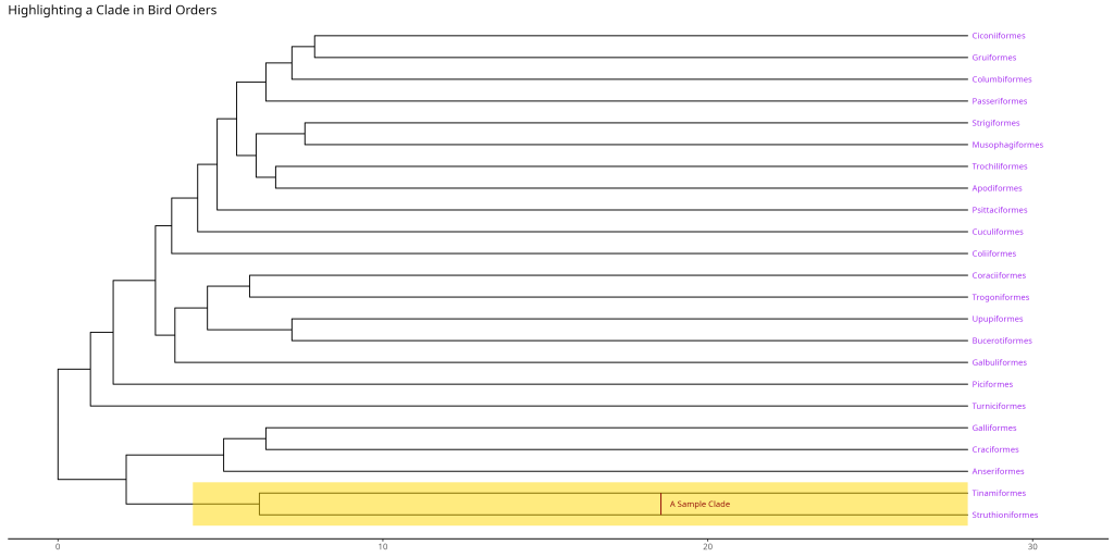

Tree Manipulations

Re-rooting Trees

Re-rooting a phylogenetic tree involves changing the position of the root, which can be important for several reasons:

• Outgroup rooting: When you have a known outgroup (a species or group that diverged before your study group), you can use it to root the tree
• Hypothesis testing: Different root positions can represent different evolutionary scenarios
• Visualization: Some root positions may make the tree easier to interpret

In our example, we’re re-rooting the bird orders tree using Struthioniformes (ostriches) as the outgroup.

# Example: Rooting the bird.orders tree on a specific outgroup
# Let's say 'Struthioniformes' (node 20 based on its label) is our outgroup
node_outgroup_bird <- which(bird.orders$tip.label == "Struthioniformes")
bird_orders_rerooted <- ape::root(bird.orders, outgroup = node_outgroup_bird, resolve.root = TRUE)

ggtree::ggtree(bird_orders_rerooted) +
  ggtree::geom_tiplab(size = 3) +
  labs(title = "Bird Orders Rerooted on Struthioniformes") +
  xlim(NA, max(fortify(bird_orders_rerooted)$x) * 1.1) +
  ggtree::theme_tree2()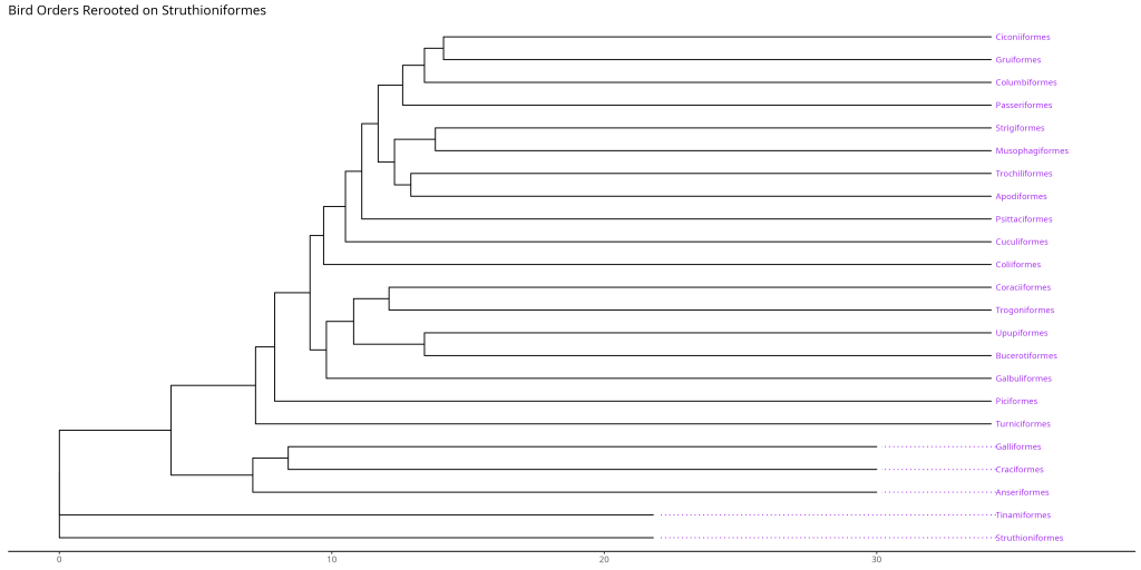

Summary and Best Practices

When working with phylogenetic trees in R, remember these key points:

• Use ape for basic tree manipulation and simple visualizations
• Use ggtree for publication-quality figures and complex annotations
• Choose the appropriate layout based on your data and research question
• Include scale bars when showing evolutionary distances
• Use highlighting and annotations strategically to emphasize important relationships

Remember that the goal of phylogenetic tree visualization is to clearly communicate evolutionary relationships. Choose your visualization style based on what aspects of the tree you want to emphasize.

Further Resources

• The ggtree Book: Comprehensive documentation of ggtree
• ape Documentation: Detailed information about the ape package
• R Project: General R programming resources