Before proceeding, ensure you have installed the R packages used in this tutorial, such as lterdatasampler, ggpubr, dplyr, and ggthemes. You can install them using install.packages("package_name") in your R console.

It is generally best in statistics, especially when starting out on our own individual journeys as statisticians, to choose the simplest test that A) will answer our question, and B) we can satisfy the assumptions of.

When comparing two sample means, the standard test to perform here is the two-sample t-test. The test statistic is calculated as:

t = \frac{(\bar{Y_1} - \bar{Y_2}) - (\mu_1 - \mu_2)_0}{SE_{Y_1 - Y_2}}

This test assumes three major things:

1. Normality: Data in each group are approximately normally distributed.
2. Homoskedasticity: (Equality of variances) Data in each group have approximately the same variance.
3. Independence: The samples are independent. This means the observations in one group are not related to or influenced by observations in the other group, and observations within each group are also independent of each other (e.g., one crab’s size doesn’t affect another crab’s size within the same sample). This assumption is primarily met through careful study design and data collection procedures, ensuring that the selection of one subject or measurement does not influence another. Unlike normality or homoskedasticity, it’s not typically assessed with a post-hoc statistical test on the data itself but is a fundamental aspect of how the data were gathered.

Our question is simply that we believe there is a size difference between crabs from different locations. Let’s start by attempting to justify these assumptions, and if we can, using the simple test.

Two-sided T-tests

We’ll use data on crab sizes:

library(tidyverse)
library(lterdatasampler)

crab_sizes <- lterdatasampler::pie_crab
crab_sizes

## tibble [392 × 9] (S3: tbl_df/tbl/data.frame)
##  $ date         : Date[1:392], format: "2016-07-24" "2016-07-24" "2016-07-24" "2016-07-24" ...
##  $ latitude     : num [1:392] 30 30 30 30 30 30 30 30 30 30 ...
##  $ site         : Factor w/ 13 levels "BC","CC","CT",..: 5 5 5 5 5 5 5 5 5 5 ...
##  $ size         : num [1:392] 12.4 14.2 14.5 12.9 12.4 ...
##  $ air_temp     : num [1:392] 21.8 21.8 21.8 21.8 21.8 ...
##  $ air_temp_sd  : num [1:392] 6.39 6.39 6.39 6.39 6.39 ...
##  $ water_temp   : num [1:392] 24.5 24.5 24.5 24.5 24.5 ...
##  $ water_temp_sd: num [1:392] 6.12 6.12 6.12 6.12 6.12 ...
##  $ name         : Factor w/ 13 levels "Bare Cove Park",..: 4 4 4 4 4 4 4 4 4 4 ...

There are a number of sites in this dataset, so let’s compare crabs from two northern sites and two southern sites. Our northern sites will be “Cape Cod” and “Narragansett Bay NERR” and our southern sites will be “Guana Tolomoto Matanzas NERR” and “Sapelo Island NERR”.

It’s important to never forget the underlying mathematics of what we’re doing, we should never simply rely on our computers exclusively and not understand what we’re doing, so let’s review the equations underlying the t-test. We’ll be calculating the test statistic \(t\) as described above. As we are testing a hypothesis that the sizes are different, we can state this formally as \(H_0: \mu_1 = \mu_2\) and \(H_a: \mu_1 \neq \mu_2\).

Since we stated we believe \(H_0: \mu_1 = \mu_2\), this is a two-sided test, we have not suggested that \(\mu_1 > \mu_2\) or \(\mu_1 < \mu_2\).

Assumptions of the Test

Before we proceed we need to take into account assumptions of our chosen test. We’ll assume our samples are independent (that is, that we’ve selected samples that aren’t related), but our two-sample t-test requires two other things:

1. normality
2. homoskedasticity.

Normality

To assess the normality of our data, let’s first inspect it visually and then double-check with a statistical test of normality (the Shapiro-Wilks test). We will use ggplot2 for plotting.

Let’s use a density plot to check if the data follow the normal/Gaussian curve:

bind_rows(crab_sizes_north, crab_sizes_south) %>%
  ggplot(aes(x = size, fill = Group)) +
  geom_density(alpha = 0.5) +
  labs(
    x = "Crab Size (mm)",
    y = "Density"
  ) +
  ggthemes::theme_base()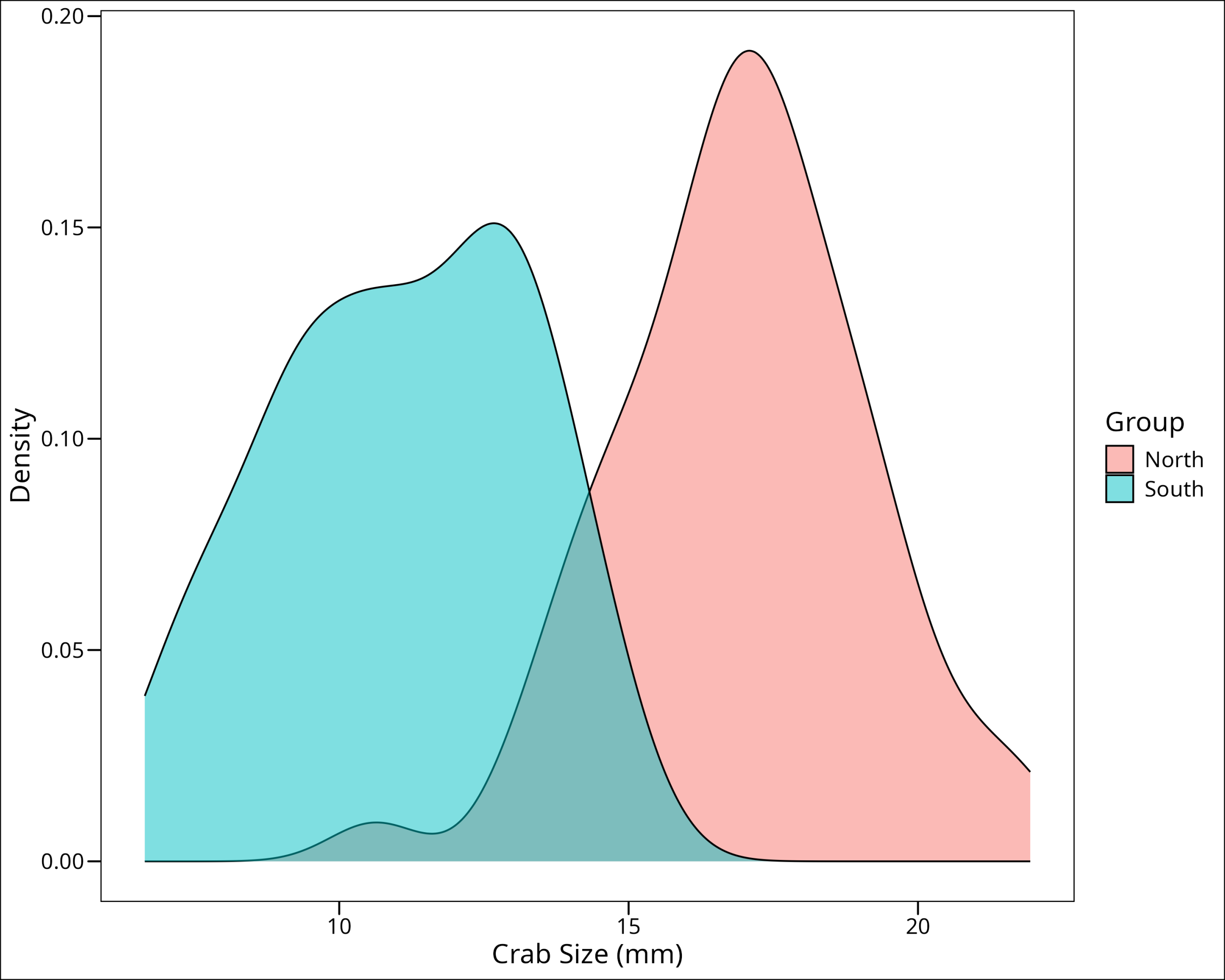

They both look normal. Let’s look at the QQ plots:

bind_rows(crab_sizes_north, crab_sizes_south) %>%
  ggplot(aes(sample = size, color = Group)) +
  geom_qq() +
  geom_qq_line() +
  ggthemes::theme_base() +
  labs(
    x = "Theoretical Quantiles",
    y = "Sample Quantiles"
  )

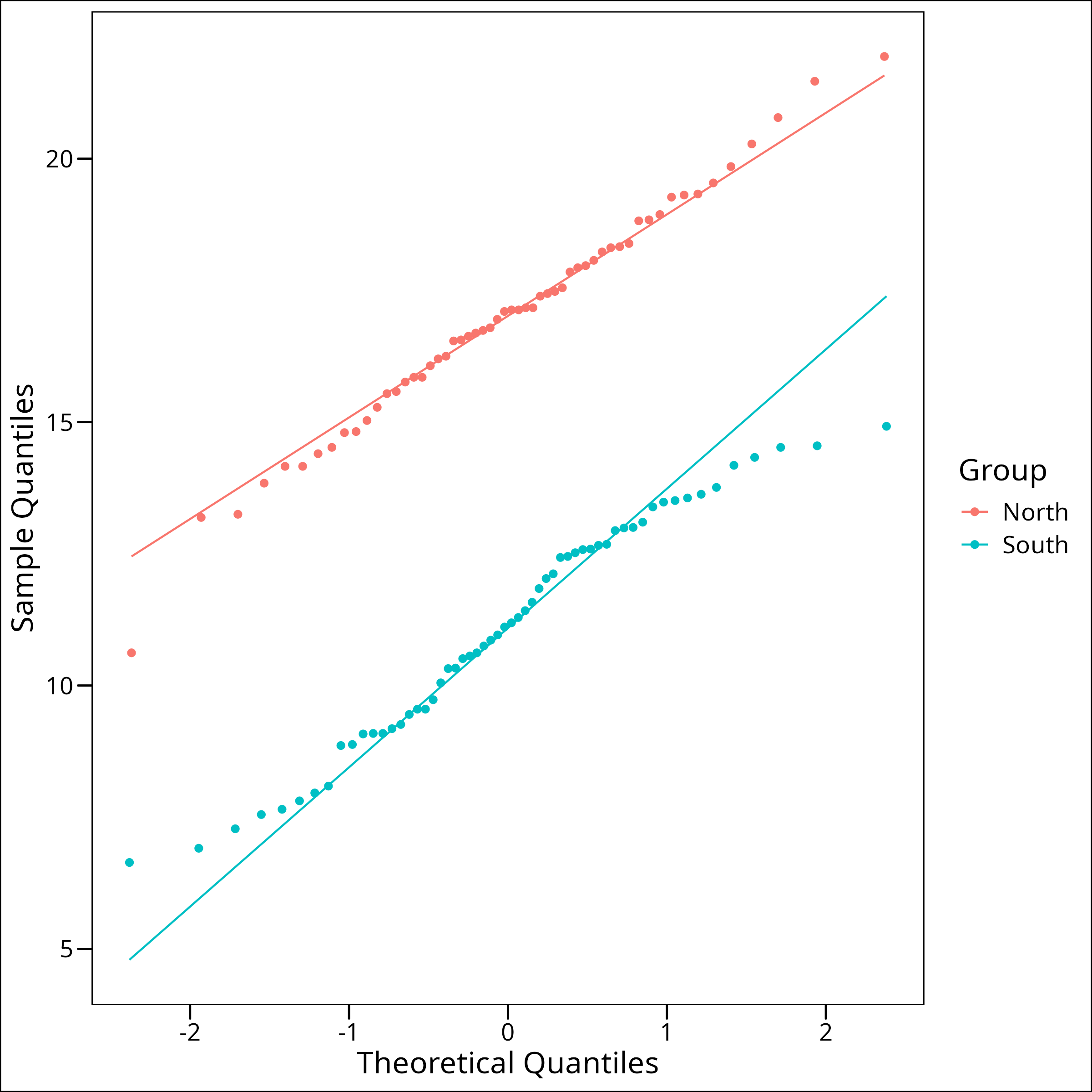
We’re looking for the points to follow the black line and for no points to be outside the grey error bars. Both of these look pretty good. It’s worth noting that while for our purposes we can simply use plots to check for normality, it can sometimes be helpful to use a statistical test to check for normality. Since we’re using a t-test, this isn’t necessary as they can be robust to some degree of non-normality, but if strict normality is required, it’s possible to use a Shapiro-Wilk’s test. A Shapiro-Wilk’s test is a significance test that has a null hypothesis of normality. If the test is SIGNIFICANT then the test has indicated there is non-normality in the data.

We can do this in R very easily. The function shapiro.test() comes shipped in core R with the stats package. First for the northern sites:

stats::shapiro.test(crab_sizes_north$size)

## 	Shapiro-Wilk normality test
## 
## data:  crab_sizes_north$size
## W = 0.99161, p-value = 0.9644

Okay, and we see that our p-value is > 0.05 so we’ll fail to reject the null. For the southern sites:

stats::shapiro.test(crab_sizes_south$size)

## 	Shapiro-Wilk normality test
## 
## data:  crab_sizes_south$size
## W = 0.96787, p-value = 0.1269

Here we see a large p-value, >> 0.05, so again we fail to reject the null.

Good, we’ve satisfied the condition of normality.

Homoskedasticity (Equality of Variances)

Our second assumption for the two-sample t-test is that the variances of the two groups are equal (homoskedasticity). If the variances are significantly different (heteroskedasticity), we should use a variation of the t-test that doesn’t assume equal variances (like Welch’s t-test, by setting var.equal = FALSE in R’s t.test() function).

We can formally test for equality of variances using an F-test, which is performed by the var.test() function in R. The null hypothesis for this test is that the variances are equal. If the test outcome is SIGNIFICANT, it means we have unequal variances.

# Test for equality of variances (Homoskedasticity)
# H0: The variances are equal
# Ha: The variances are not equal
var_test_result <- stats::var.test(crab_sizes_north$size, crab_sizes_south$size)
var_test_result

## 	F test to compare two variances
## 
## data:  crab_sizes_north$size and crab_sizes_south$size
## F = 0.97195, num df = 55, denom df = 57, p-value = 0.9169
## alternative hypothesis: true ratio of variances is not equal to 1
## 95 percent confidence interval:
##  0.5732314 1.6521757
## sample estimates:
## ratio of variances
##          0.9719504

Interpreting this output: The p-value (0.9169) is much greater than the common significance level of 0.05. Therefore, we fail to reject the null hypothesis that the variances are equal. The F-statistic is 0.97195, and the 95% confidence interval for the ratio of variances (0.573 to 1.652) includes 1, which is consistent with the variances being equal.

Visually, we can also compare the spread of data in boxplots for the two groups. If the interquartile ranges and overall spread look reasonably similar, it provides some support for the homoskedasticity assumption.

# Visual check with boxplots
bind_rows(crab_sizes_north, crab_sizes_south) %>%
  ggplot(aes(x = Group, y = size, fill = Group)) +
  geom_boxplot() +
  ggthemes::theme_base() +
  labs(
    x = "Geographic Region",
    y = "Crab Size (mm)"
  )

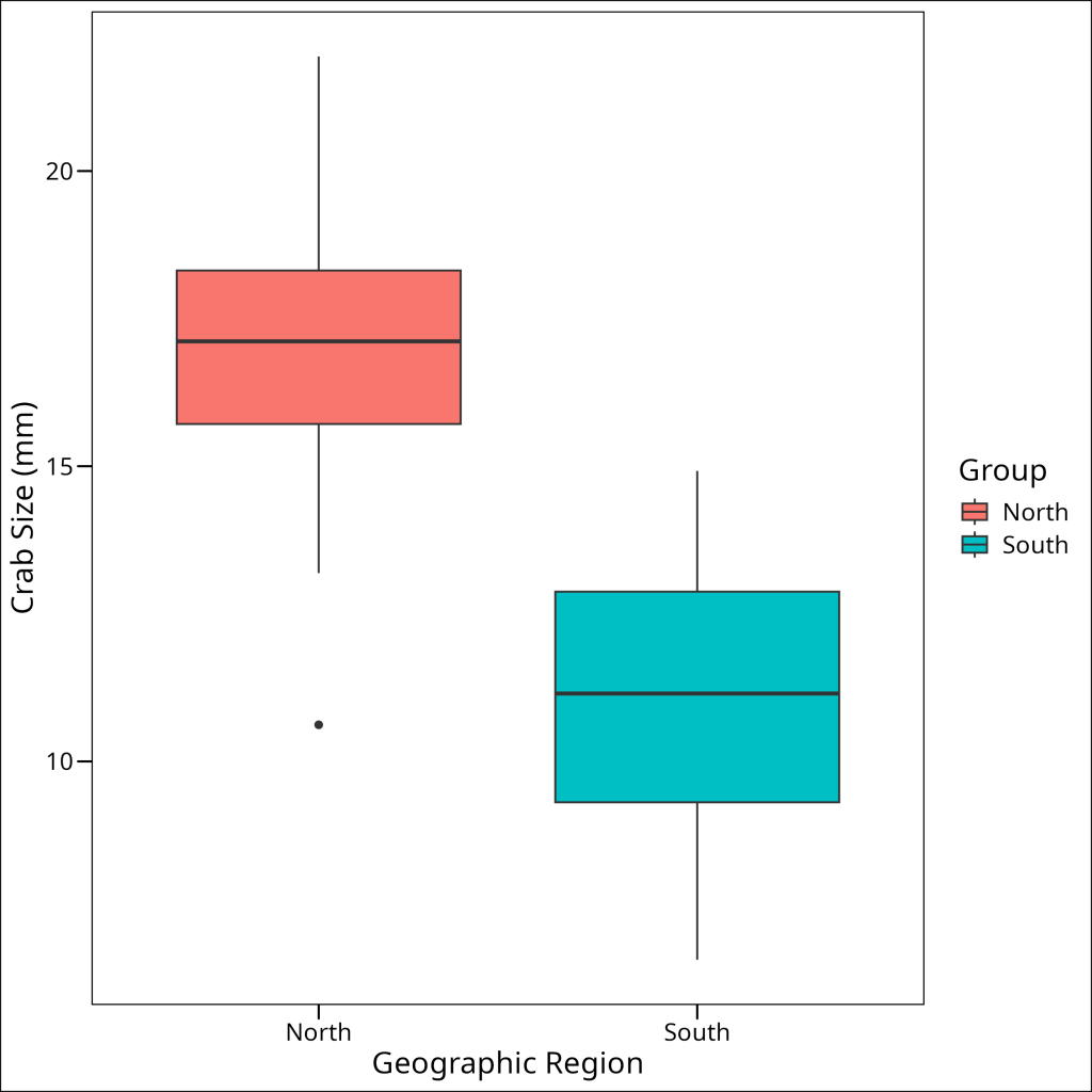
Indeed, the boxplots verify that we have similar spread in each of the subsets.

The test

So now we can actually perform the test. It’s quite simple, we’ll use the t.test() function:

t_test_res <- stats::t.test(
  crab_sizes_north$size, # sample of group 1
  crab_sizes_south$size, # sample of group 2
  var.equal = TRUE # Regular t-test or Welch's t-test depending on the variance
)
t_test_res

## 	Two Sample t-test
## 
## data:  crab_sizes_north$size and crab_sizes_south$size
## t = 14.436, df = 112, p-value < 2.2e-16
## alternative hypothesis: true difference in means is not equal to 0
## 95 percent confidence interval:
##  5.089136 6.708352
## sample estimates:
## mean of x mean of y 
##  16.98357  11.08483

We see our result here, and it turns out the p-value is very small (p < 2.2e-16), so we can reject the null hypothesis. There is good evidence that \(\mu_1 \neq \mu_2\) (i.e., the mean crab sizes in the northern and southern regions are different). The t-statistic is 14.436 with 112 degrees of freedom. The 95% confidence interval for the difference in means is (5.09, 6.71), which does not include 0, further supporting the rejection of H₀. The sample mean for northern crabs is about 17.0mm and for southern crabs is about 11.1mm.

One-sided T-tests

In our above example we stated our hypothesis such that we could use a two-sided test. But what if when we were formulating our hypotheses, we’d said we believe the southern crabs would be bigger? Note that we’re pretending here that we HAVEN’T seen the results just above, since that would be p-hacking. But let’s say we thought “Hey, warmer water, lots of sun, maybe more beaches, that could mean bigger crabs.” (I stress this is not an intelligently derrived biological hypothesis).

But in this case, we could perform the exact test as above, but instead determine that we wanted a one-sided test. That’s easy enough and uses all the same code, with one additional argument. Using the same dataset, we would simply add an argument for alternative. The syntax here is saying that in the function, we pass two sets of numbers, x and y. If we believe x to be less than y, we pass “less”, and if we believe x to be greater than y, then we pass “greater”.

In our case, we are hypothesizing that the southern crabs (crab_sizes_south) are greater in size than the northern crabs, so let’s set x to be the crab_sizes_south and the y to be crab_sizes_north, and then alternative = "greater", so this is testing the alternate hypothesis that \(\mu_{south} > \mu_{north}\):

t_test_oneside_res <- stats::t.test(
  crab_sizes_south$size,
  crab_sizes_north$size,
  var.equal = TRUE,
  alternative = "greater"
)
t_test_oneside_res

## 	Two Sample t-test
## 
## data:  crab_sizes_south$size and crab_sizes_north$size
## t = -14.436, df = 112, p-value = 1
## alternative hypothesis: true difference in means is greater than 0
## 95 percent confidence interval:
##  -6.576453       Inf
## sample estimates:
## mean of x mean of y
##  11.08483  16.98357

So we see here we have a p-value of 1. Given that we do know which group is actually bigger (North: ~17.0mm, South: ~11.1mm, from our previous two-sided test), this result from testing \(H_a: \mu_{south} > \mu_{north}\) (i.e., testing if southern crabs are larger than northern crabs) is not surprising. We fail to reject the null hypothesis (\(H_0: \mu_{south} = \mu_{north}\)) against our stated alternative (\(H_a: \mu_{south} > \mu_{north}\)). This simply means we found no evidence to support the specific claim that southern crabs are larger than northern crabs. It does not mean we accept the null hypothesis, nor does it imply that northern crabs are definitively larger (though our earlier two-sided test did suggest a significant difference where northern crabs were larger).

What to do with non-normality?

Going back to our assumptions, let’s re-start our process of this test but with a different grouping of data.

What if we just took the MOST northern and southern sites alone, not groups of sites, and did a t-test on those two? say that instead of the two sites acting as our “northern” sites, we chose to use the single most northern site: “Plum Island Estuary – West Creek” (PIE), and for our southern site, we took the most southern one – “Guana Tolomoto Matanzas NERR” (GTM). If we start again by checking our assumptions, we would first have to check for normality of both our groups.

Let’s start by again dividing our data:

crab_sizes_s_GTM <- crab_sizes %>%
  filter(site == "GTM")
crab_sizes_n_PIE <- crab_sizes %>%
  filter(site == "PIE")

You know the drill by now, let’s visualize some density plots and QQ plots:

bind_rows(crab_sizes_s_GTM, crab_sizes_n_PIE) %>%
  ggplot(aes(x = size, fill = site)) +
  geom_density(alpha = 0.5) +
  labs(
    x = "Crab Size (mm)",
    y = "Density"
  ) +
  ggthemes::theme_base()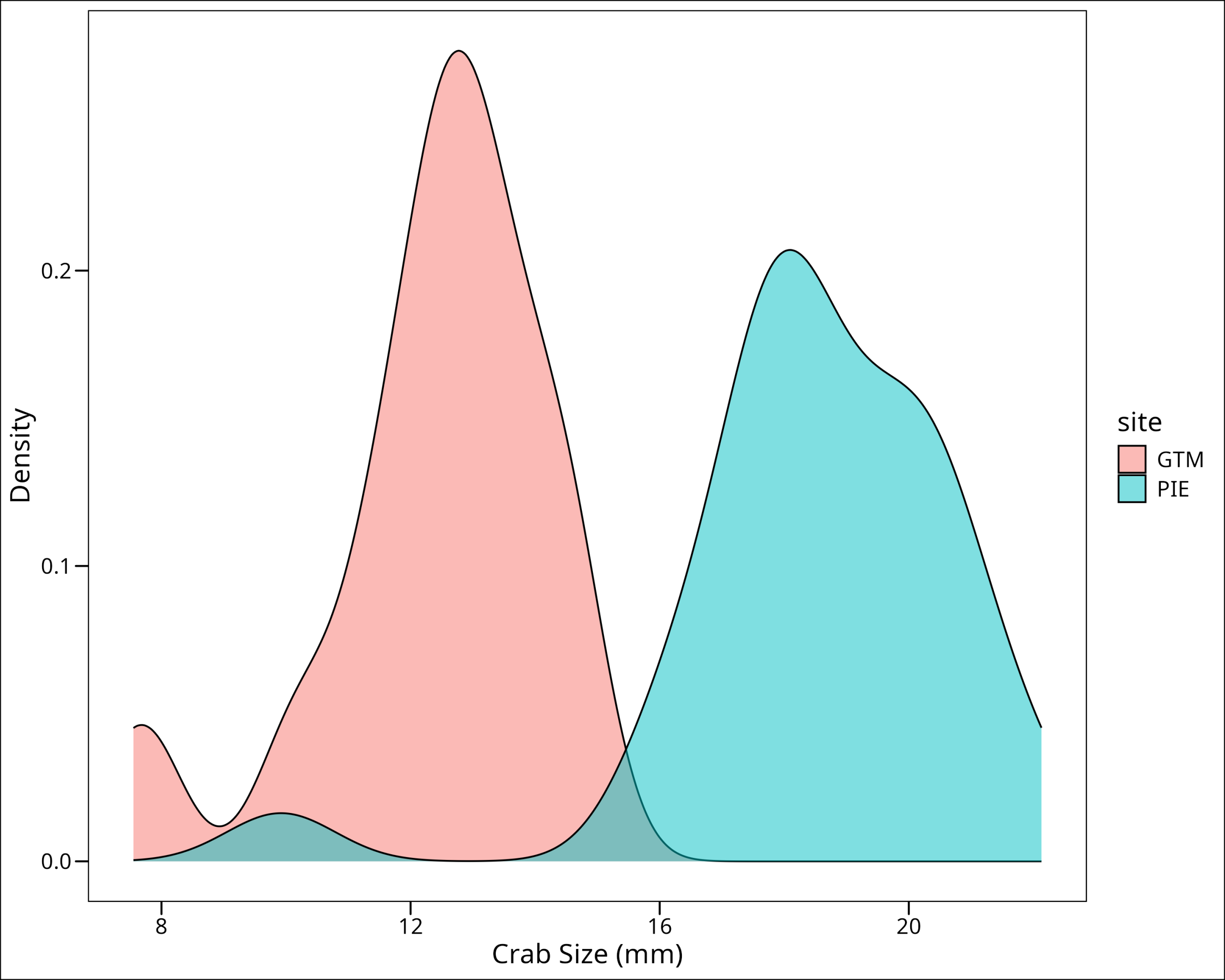

Uh oh! Notice that in both GTM and PIE groups, we have a small subset of outliers manifesting as a hump of lower values. Let’s check what the impact is on the QQ plot:

bind_rows(crab_sizes_s_GTM, crab_sizes_n_PIE) %>%
  ggplot(aes(sample = size, color = site)) +
  geom_qq() +
  geom_qq_line() +
  ggthemes::theme_base() +
  labs(
    x = "Theoretical Quantiles",
    y = "Sample Quantiles"
  )

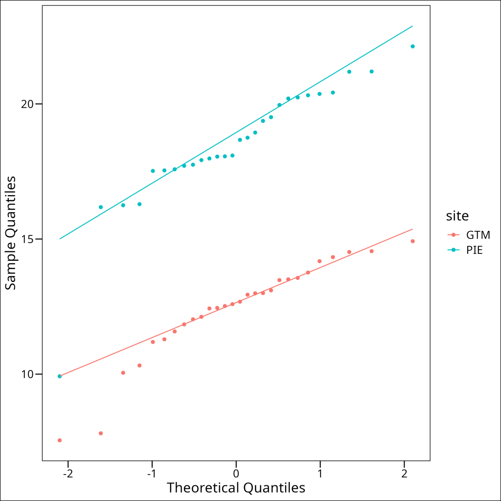
Indeed, we can see that there are deviations from an ideal normal distribution in both groups:

• For the PIE group, there is a trend towards sample quantiles shifting to be lower than their theoretical counterparts (i.e. datapoints aim to be below the QQ line) and the lowest quantile is far below the QQ line (see single blue point on that blends with the GTM QQ line).
• For the GTM group, the lower set of sample quantiles are far lower than their expected theoretical counterparts and therefore dip far below the QQ line.

In all likeliness these groups do not meet the normality assumption. Let’s confirm with Shapiro-Wilk tests:

stats::shapiro.test(crab_sizes_s_GTM$size)

## 
## 	Shapiro-Wilk normality test
## 
## data:  crab_sizes_s_GTM$size
## W = 0.90078, p-value = 0.01193

stats::shapiro.test(crab_sizes_n_PIE$size)

## 
## 	Shapiro-Wilk normality test
## 
## data:  crab_sizes_n_PIE$size
## W = 0.84894, p-value = 0.0008899

For the GTM site, the p-value is 0.01193, and for the PIE site, the p-value is 0.0008899. Both are less than the typical significance level of 0.05, leading us to reject the null hypothesis of normality for both datasets. This means a t-test is not appropriate here, and we should consider a non-parametric alternative.

Non-Parametric Tests

The best alternative for our case is the Mann-Whitney U Test.

There are a few things to note about this test however. This test actually does NOT compare sample means. The Mann-Whitney’s stated use is to determine whether or not the groups or samples are drawn from equal populations, that is, are the shape of the data the same. It can be interpreted that this is analogous to saying the median values are the same for both groups.

Assumptions

Just because the data do not have to be normal, there are still important assumptions we need to satisfy. The data still need to be independent, but there are two additional assumptions:

1. The variable needs to be continuous
2. The data are assumed to be similar in shape

The second assumption here is important! While the data do not have to be normal, they have to exhibit a similar skew.

Continuity

We know that our variable is continuous, so this assumption is met.

Skew

Measuring a degree of skew can be subjective. However, looking back at the density plots we created for the GTM (crab_sizes_s_GTM$size) and PIE (crab_sizes_n_PIE$size) sites when checking for normality, we can visually assess if their shapes are roughly similar. Both distributions appeared somewhat left-skewed. For the Mann-Whitney U test to be most accurately interpreted as a test of medians, the shapes of the distributions should be similar. If they are not, the test is still valid for assessing if one distribution is stochastically greater than the other, but the interpretation regarding medians becomes less direct. For this tutorial, we will proceed based on the visual assessment that the distributions, while not normal, have a generally similar skewed shape.

The test

The Mann-Whitney is sometimes referred to as the Mann-Whitney-Wilcoxon test, and so is performed using the wilcox.test() function, again from stats:

stats::wilcox.test(crab_sizes_s_GTM$size,
                  crab_sizes_n_PIE$size)

## 
## 	Wilcoxon rank sum exact test
## 
## data:  crab_sizes_s_GTM$size and crab_sizes_n_PIE$size
## W = 26, p-value = 3.068e-12
## alternative hypothesis: true location shift is not equal to 0

Here we see our p-value is << 0.05, so we can reject our null hypothesis that say that these two medians are equal, and thus conclude (generally) that the northern and southern populations have different sizes. Note again that this is a two-sided test so we’re not testing directionality.