Why Do We Need Confidence Intervals?

When we take a sample from a population – say, measuring the heights of 100 randomly selected trees in a forest – and calculate the average height, we get a sample mean. This sample mean is our best estimate of the true population mean height of all trees in that forest. However, if we were to take a different sample of 100 trees, we would likely get a slightly different sample mean. This variability is inherent in sampling.

A point estimate (like the sample mean) alone doesn’t tell us how precise that estimate is. Is the true population mean likely to be very close to our sample mean, or could it be quite different? A confidence interval (CI) addresses this by providing a range of plausible values for the true population parameter, based on our sample data and a chosen level of confidence.

The Normal Distribution and the 68-95-99.7 Rule

Recall from our discussion on sampling distributions that the Central Limit Theorem tells us that the distribution of sample means tends to be approximately normal, especially as sample size increases, regardless of the shape of the population distribution. This normality is key to constructing confidence intervals.

A useful property of the normal distribution is the 68-95-99.7 rule (also known as the empirical rule). It states that for a normal distribution:

• Approximately 68% of the data falls within 1 standard deviation (\(\sigma\)) of the mean (\(\mu\)).
• Approximately 95% of the data falls within 2 standard deviations (\(2\sigma\)) of the mean.
• Approximately 99.7% of the data falls within 3 standard deviations (\(3\sigma\)) of the mean.

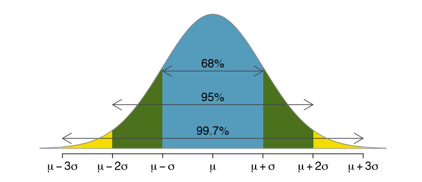
This rule provides a conceptual bridge to understanding confidence levels. For instance, the “95%” part is directly related to the commonly used 95% confidence interval, suggesting that values within about two standard deviations (more precisely, 1.96 standard deviations for a 95% CI) of the sample mean are considered plausible for the population mean.

What is a Confidence Interval?

A confidence interval (CI) is a range of values, derived from sample statistics, that is likely to contain the value of an unknown population parameter. It is expressed in terms of a confidence level, most commonly 95%, but other levels like 90% or 99% are also used.

Important Interpretation: A 95% confidence interval means that if we were to take many random samples from the same population and construct a 95% CI for each sample, about 95% of those intervals would capture the true population parameter. It does not mean there is a 95% probability that the true population parameter lies within a particular calculated CI. Once a CI is calculated, the true parameter either is in it or it isn’t; the probability refers to the long-run success rate of the method.

Common misconceptions to avoid:

• A 95% CI does NOT mean that 95% of the sample data fall within the interval.
• A 95% CI is NOT a range that has a 95% chance of containing the true parameter for that specific interval (the parameter is fixed, the interval varies with the sample).

Calculating a Confidence Interval for a Population Mean (\(\mu\))

The formula for a confidence interval for a population mean (\(\mu\)) depends on whether the population standard deviation (\(\sigma\)) is known or unknown.

Case 1: Population Standard Deviation (\(\sigma\)) is Known

This scenario is rare in practice because we seldom know the true population standard deviation. However, it’s a good starting point for understanding the concepts. When \(\sigma\) is known and the sampling distribution of the mean is normal (or approximately normal by the Central Limit Theorem), the CI is calculated as:

\text{CI} = \bar{x} \pm z \cdot \frac{\sigma}{\sqrt{n}}

Where:

• \(\bar{x}\) is the sample mean.
• \(z\) is the z-score from the standard normal distribution corresponding to the desired confidence level (e.g., for a 95% CI, \(z \approx 1.96\); for a 90% CI, \(z \approx 1.645\); for a 99% CI, \(z \approx 2.576\)). This z-score defines how many standard errors wide the interval is.
• \(\sigma\) is the known population standard deviation.
• \(n\) is the sample size.
• \(\frac{\sigma}{\sqrt{n}}\) is the standard error of the mean (SEM) when \(\sigma\) is known.

Case 2: Population Standard Deviation (\(\sigma\)) is Unknown

This is the much more common scenario. When \(\sigma\) is unknown, we estimate it using the sample standard deviation (\(s\)). This introduces additional uncertainty, so instead of the z-distribution, we use the t-distribution. The t-distribution is similar in shape to the normal distribution (bell-shaped and symmetric) but has heavier tails, meaning it accounts for the greater uncertainty, especially with smaller sample sizes. The shape of the t-distribution depends on the degrees of freedom (df), which for a CI of a single mean is \(n-1\).

The CI formula becomes:

\text{CI} = \bar{x} \pm t \cdot \frac{s}{\sqrt{n}}

Where:

• \(\bar{x}\) is the sample mean.
• \(t\) is the t-value (critical value) from the t-distribution with \(n-1\) degrees of freedom for the desired confidence level. This value can be found using statistical tables or R functions like qt().
• \(s\) is the sample standard deviation.
• \(n\) is the sample size.
• \(\frac{s}{\sqrt{n}}\) is the estimated standard error of the mean (SEM).

R Example: Calculating CI for a Mean (\(\sigma\) Unknown)

Let’s illustrate this with a small R example. Suppose we have a sample of 10 tree height measurements (in meters):

# Sample data: heights of 10 trees
set.seed(42) # for reproducibility
tree_heights <- round(rnorm(n = 10, mean = 20, sd = 3), 1)
tree_heights

[1] 24.1 18.3 21.1 21.9 21.2 19.7 24.5 19.7 26.1 19.8

First, calculate the sample mean (\(\bar{x}\)) and sample standard deviation (\(s\)):

sample_mean <- mean(tree_heights)
sample_sd <- sd(tree_heights)
n <- length(tree_heights)

sample_mean
sample_sd
n

[1] 21.64
[1] 2.51
[1] 10

Next, find the t-value for a 95% confidence interval with \(n-1 = 9\) degrees of freedom. For a 95% CI, we need 2.5% in each tail (0.025). The qt() function gives us the t-value for a given lower tail probability.

alpha <- 0.05 # Significance level for 95% CI
df <- n - 1
t_value <- qt(1 - alpha/2, df) # Gets the t-value for the upper tail (1 - 0.025 = 0.975)
t_value

[1] 2.262157

Now, calculate the margin of error (ME) and the CI:

margin_of_error <- t_value * (sample_sd / sqrt(n))
margin_of_error

lower_bound <- sample_mean - margin_of_error
upper_bound <- sample_mean + margin_of_error

lower_bound
upper_bound

[1] 1.576215
[1] 19.63379
[1] 22.78621

So, the 95% confidence interval for the true mean tree height is approximately (19.63, 22.79) meters.

R can calculate this directly using the t.test() function:

t_test_result <- t.test(tree_heights)
t_test_result$conf.int

[1] 19.63379 22.78621
[1] 0.95

The results match our manual calculation!

Interpreting Confidence Intervals Correctly

It is crucial to interpret CIs correctly. For our example, the 95% CI for tree height is (19.63m, 22.79m). This means:

• We are 95% confident that the true mean height of all trees in the population from which our sample was drawn lies between 19.63m and 22.79m. The term “confident” here refers to the reliability of the method used to create the interval.
• If we were to repeat this sampling process many times (drawing many different samples from the same population and calculating a 95% CI for each), we would expect about 95% of these constructed intervals to successfully capture the true, fixed population mean height. Our specific interval (19.63m, 22.79m) is one of these many possible intervals.

What it does not mean, and why “confidence” is different from “probability” in this context:

• It does NOT mean there is a 95% probability that the true population mean lies within this specific, already calculated interval (19.63m, 22.79m). The true population mean is a already fixed value (fixed values do not have a probability); it doesn’t vary. Once our sample is taken and the interval is calculated, the true mean either is within this specific interval or it is not. There isn’t a 95% chance it’s hopping in or out of this particular range. The 95% applies to the success rate of the procedure of generating such intervals over many hypothetical repetitions, not to a single instance.
• It does NOT mean that 95% of the individual tree heights in the sample or population fall within this range. The CI is for the population mean, not individual data points.

Factors Affecting the Width of a Confidence Interval

The width of a confidence interval reflects the precision of our estimate. A narrower interval suggests a more precise estimate of the population parameter, while a wider interval indicates less precision. Three main factors influence the width of a CI for a population mean:

1. Confidence Level: A higher confidence level (e.g., 99% vs. 95%) results in a wider interval. To be more confident that the interval captures the true parameter, we need to include a wider range of plausible values. This means a larger z-score or t-value is used in the calculation.
2. Sample Size (\(n\)): A larger sample size leads to a narrower interval. As \(n\) increases, the standard error of the mean (\(s/\sqrt{n}\)) decreases, indicating that our sample mean is likely to be closer to the true population mean.
3. Sample Variability (\(s\)): Greater variability in the sample data (a larger sample standard deviation \(s\)) leads to a wider interval. If the data points themselves are more spread out, there’s more uncertainty about the true population mean.

R Example: Impact of Sample Size on CI Width

Let’s see how sample size affects the CI width. We’ll simulate two datasets with the same underlying mean and standard deviation, but different sample sizes.

set.seed(123) # For reproducibility
# Small sample
data_small_n <- rnorm(n = 15, mean = 50, sd = 10)
ci_small_n <- t.test(data_small_n)$conf.int
width_small_n <- ci_small_n[2] - ci_small_n[1]

# Larger sample
data_large_n <- rnorm(n = 100, mean = 50, sd = 10)
ci_large_n <- t.test(data_large_n)$conf.int
width_large_n <- ci_large_n[2] - ci_large_n[1]

cat("95% CI for small sample (n=15): (", round(ci_small_n[1],2), ", ", round(ci_small_n[2],2), ") -> Width: ", round(width_small_n,2), "\n")
cat("95% CI for large sample (n=100): (", round(ci_large_n[1],2), ", ", round(ci_large_n[2],2), ") -> Width: ", round(width_large_n,2), "\n")

95% CI for small sample (n=15): ( 44.39 , 54.9 ) -> Width:  10.51 
95% CI for large sample (n=100): ( 48.01 , 52.04 ) -> Width:  4.03 

As expected, the confidence interval for the larger sample (n=100) is narrower than for the smaller sample (n=15), indicating a more precise estimate of the population mean when more data is available.

Conclusion

Confidence intervals are a fundamental tool in statistics for expressing the uncertainty associated with sample estimates. They provide a range of plausible values for an unknown population parameter, such as the population mean, based on sample data. Understanding how to calculate, interpret, and recognize the factors that influence CIs is crucial for drawing meaningful conclusions from data in ecology, evolutionary biology, and beyond. By always reporting CIs alongside point estimates, we present a more complete picture of our findings and acknowledge the inherent variability in statistical estimation.