After fitting statistical models like ANOVA, linear regression, GLMs, or mixed-effects models, we often want to ask more specific questions than the overall model summary provides. For instance, a significant F-test in an ANOVA tells us that at least one group differs from another, but it doesn’t tell us which specific groups differ. Similarly, regression coefficients tell us about the effect of a predictor compared to a reference level, but we might be interested in comparing other levels or combinations of levels directly. This is where contrasts and post-hoc testing become essential.

Introduction

Contrasts are essentially planned comparisons between specific means or combinations of means within our model. They allow us to test precise hypotheses derived from our research questions. For example, if we have three treatment groups (Control, Treatment A, Treatment B), we might want to compare the average outcome of the two treatment groups against the control, or compare Treatment A directly against Treatment B. Post-hoc tests are often performed after an initial significant result (like an ANOVA F-test or an assessment of the model summary) to explore which specific group differences are driving that significance, often involving multiple pairwise comparisons.

While it’s possible to calculate contrasts manually, this can become complex, especially with interaction terms or complicated models like mixed-effects models. Fortunately, the R ecosystem provides powerful tools to simplify this process. The emmeans package (Estimated Marginal MEanS) is particularly useful. It allows us to easily compute estimated marginal means (also known as least-squares means), perform various contrasts, conduct post-hoc tests, and visualize results, all while properly accounting for the model structure and potential covariates. This tutorial will introduce the concept of contrasts and demonstrate how to use the emmeans package in R to perform insightful post-hoc analyses.

Example 1: Plant Defenses in Kluane – Using `emmeans`

To illustrate how contrasts work, we’ll use data from the Kluane Boreal Forest Ecosystem Project. This long-term experiment investigated how fertilization and the exclusion of herbivores affect vegetation dynamics. The specific data we’ll analyze concerns the concentration of phenolic compounds (a measure of plant defense) in yarrow (Achillea millefolium).

The experiment involved sixteen 5x5m plots. Each plot was assigned one of four treatments: control (no manipulation), exclosure (fenced to keep herbivores out), fertilizer (N-P-K added), or both (fenced and fertilized). Each plot was then split in half. One half received its assigned treatment continuously for 20 years (“permanent” duration). The other half received the treatment for the first 10 years, after which the treatment was stopped, allowing the vegetation to revert towards its untreated state (“reverse” duration). Our goal is to understand how these treatments and their duration influenced yarrow’s phenolic concentrations.

Data Preparation and Visualization

First, let’s load the necessary libraries and the data. We’ll convert plot, treatment, and duration into factors. Notice that we use fct_relevel to set “control” as the reference level for the treatment factor, which influences how R encodes the model later.

library(tidyverse)
library(lmerTest)
library(broom.mixed) # For tidying model outputs, especially with emmeans
library(emmeans)    # For calculating estimated marginal means and contrasts

# Load the data
df_kluane <- read_csv("https://www.zoology.ubc.ca/~bio501/R/data/kluane.csv") %>%
  mutate(
    plot = as.factor(plot),
    # Set reference level to 'control'
    treatment = as.factor(treatment) %>% fct_relevel("control", "exclosure", "fertilizer", "both"),
    duration = as.factor(duration) # Levels: permanent, reverse
  )

# Check the structure
str(df_kluane)

tibble [32 × 4] (S3: tbl_df/tbl/data.frame)
 $ plot     : Factor w/ 16 levels "1","2","3","4",..: 1 1 2 2 3 3 4 4 5 5 ...
 $ treatment: Factor w/ 4 levels "control","exclosure",..: 1 1 3 3 1 1 3 3 4 4 ...
 $ duration : Factor w/ 2 levels "permanent","reverse": 1 2 1 2 1 2 1 2 1 2 ...
 $ phen.ach : num [1:32] 44 36.5 14.2 28.6 42.4 ...

Remember your training! It’s always wise to visualize the data. We’ll plot the log-transformed phenolic concentrations, faceted by treatment, showing the change between the “permanent” and “reverse” durations. Lines connect the two measurements from the same plot.

df_kluane %>%
  ggplot(aes(y = log(phen.ach), x = duration, fill = duration, color = duration)) +
  geom_line(aes(group = plot), col = "black", alpha=0.3) + # Connect points within plots
  geom_point(size = 3, position = position_dodge(width = 0.2)) + # Dodge points slightly
  facet_wrap(~treatment, nrow = 1) +
  labs(
      title = "Yarrow Phenolic Concentration by Treatment and Duration",
      x = "Treatment Duration", 
      y = "Log Phenolics Concentration (mg TAE/g DW)", 
      color = "Duration", fill = "Duration"
   ) +
  ggthemes::theme_base()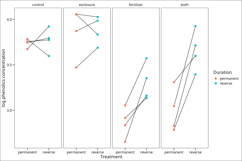

The plot suggests potential interactions. For instance, in the fertilizer and “both” treatments, phenolic concentrations seem to increase when the treatment stops (permanent –> reverse), while this pattern is less clear or absent in the control and exclosure treatments.

Fitting the Mixed-Effects Model

We expect measurements from the same plot to be correlated. Therefore, we’ll fit a linear mixed-effects model using lmer from the lmerTest package. We model log-transformed phenolics (log(phen.ach)) as a function of the interaction between treatment and duration, including plot as a random intercept to account for baseline differences between plots.

model_kluane <- lmer(
  log(phen.ach) ~ treatment * duration + (1 | plot),
  data = df_kluane
)

# Display the model summary
summary(model_kluane)

Linear mixed model fit by REML. t-tests use Satterthwaite's method ['lmerModLmerTest']
Formula: log(phen.ach) ~ treatment * duration + (1 | plot)
   Data: df_kluane

REML criterion at convergence: -1.4

Scaled residuals: 
     Min       1Q   Median       3Q      Max 
-1.55278 -0.58471  0.03425  0.52871  1.61347 

Random effects:
 Groups   Name        Variance Std.Dev.
 plot     (Intercept) 0.01292  0.1137  
 Residual             0.02413  0.1553  
Number of obs: 32, groups:  plot, 16

Fixed effects:
                                    Estimate Std. Error       df t value Pr(>|t|)    
(Intercept)                          3.74031    0.09624 21.39871  38.865  < 2e-16 ***
treatmentexclosure                   0.12388    0.13610 21.39871   0.910  0.37284    
treatmentfertilizer                 -0.87526    0.13610 21.39871  -6.431 2.06e-06 ***
treatmentboth                       -0.74732    0.13610 21.39871  -5.491 1.78e-05 ***
durationreverse                      0.03190    0.10984 12.00000   0.290  0.77648    
treatmentexclosure:durationreverse  -0.01122    0.15534 12.00000  -0.072  0.94362    
treatmentfertilizer:durationreverse  0.40963    0.15534 12.00000   2.637  0.02169 *  
treatmentboth:durationreverse        0.63438    0.15534 12.00000   4.084  0.00152 ** 
---
Signif. codes:  0 '***' 0.001 '**' 0.01 '*' 0.05 '.' 0.1 ' ' 1

Correlation of Fixed Effects:
            (Intr) trtmntx trtmntf trtmntb drtnrv trtmntx: trtmntf:
trtmntxclsr -0.707                                                 
trtmntfrtlz -0.707  0.500                                          
treatmntbth -0.707  0.500   0.500                                   
duratinrvrs -0.571  0.404   0.404   0.404                            
trtmntxcls:  0.404 -0.571  -0.285  -0.285  -0.707                   
trtmntfrtl:  0.404 -0.285  -0.571  -0.285  -0.707  0.500            
trtmntbth:d  0.404 -0.285  -0.285  -0.571  -0.707  0.500    0.500

Interpreting the Default Summary (and its Limitations)

The model summary provides estimates for the fixed effects. Understanding these requires knowing how R handles categorical predictors. By default, R uses “treatment contrasts” (confusingly named, unrelated to the contrasts we’ll discuss later). With treatment contrasts, the first level of a factor (which we set to “control” for treatment and which is “permanent” for duration by default) becomes the reference level.

Here’s how to interpret the coefficients:

(Intercept): 3.740 is the estimated mean log phenolic concentration for the reference group: treatment="control" and duration="permanent".

treatmentexclosure: 0.124 is the difference in mean log phenolics between the exclosure treatment and the control treatment, specifically when duration="permanent".

treatmentfertilizer: -0.875 is the difference between fertilizer and control when duration="permanent".

treatmentboth: -0.747 is the difference between both and control when duration="permanent".

durationreverse: 0.032 is the difference between duration="reverse" and duration="permanent", specifically for the control treatment.

treatmentexclosure:durationreverse: -0.011 is an interaction term. It represents how much the effect of switching from permanent to reverse duration *differs* in the exclosure treatment compared to the control treatment. In other words, it’s (Exclosure:Reverse – Exclosure:Permanent) – (Control:Reverse – Control:Permanent).

treatmentfertilizer:durationreverse: 0.410 is an interaction term comparing the duration effect in the fertilizer treatment to the duration effect in the control treatment.

treatmentboth:durationreverse: 0.634 is the interaction term comparing the duration effect in the both treatment to the duration effect in the control treatment.

While informative, this summary can’t directly answer many biologically relevant questions. For example:

1. What is the estimated mean phenolic concentration for the fertilizer group under the reverse duration? (We only get the difference relative to control permanent).

2. Is the mean phenolic concentration in the “both” treatment under the reverse duration significantly different from the fertilizer treatment under the reverse duration?

3. Is the effect of switching from permanent to reverse duration significantly different between the “fertilizer” and “both” treatments? (The summary only gives comparisons relative to control).

4. Is the average phenolic concentration for a specific group (e.g., fertilizer-reverse) significantly different from a specific hypothesized value (e.g., 3.0)?

To answer these kinds of targeted questions, we need to perform specific comparisons or contrasts, which is where the emmeans package comes in.

Using `emmeans` for Specific Comparisons

The emmeans package calculates “Estimated Marginal Means” (EMMs), which are essentially model-predicted means for different groups or combinations of factor levels, averaged over any covariates. It provides a flexible framework for performing various types of contrasts based on these EMMs.

1. One-Sample Comparisons: Testing Against a Specific Value

Sometimes, we want to test if the mean of a specific group differs from a known or hypothesized value. Let’s address Question 4 from before: Is the mean log phenolic concentration of the fertilizer plots under the ‘reverse’ duration significantly greater than 3?

We use the emmeans() function, specifying the model and the factors involved (~ treatment * duration). The at argument filters the results to only the combination we care about (treatment = "fertilizer" and duration = "reverse"). We set our null hypothesis value with null = 3 and specify a one-sided test (side = "right") because we’re interested if the concentration is *greater* than 3. Finally, broom.mixed::tidy() cleans up the output to include p-values of interest.

# Q: Is fertilizer-reverse > 3?
emmeans(
  model_kluane,           # The fitted model
  ~ treatment * duration, # Specify factors involved
  at = list(treatment = c("fertilizer"), duration = "reverse"),  # Filter to the specific group of interest
  null = 3,               # Null hypothesis value
  adjust = "none",      # No adjustment needed for a single test
  side = "right"          # One-sided test (greater than)
) %>%
  broom.mixed::tidy()     # Tidy the output

# A tibble: 1 × 8
  treatment  duration estimate std.error    df  null statistic p.value
  <chr>      <chr>       <dbl>     <dbl> <dbl>     <dbl>   <dbl>
1 fertilizer reverse      3.31    0.0962  21.4     3      3.19 0.00219

The output shows an estimated mean log phenolic concentration of 3.31 for this group. The p-value (0.00219) is less than the conventional alpha level of 0.05, suggesting strong evidence against the null hypothesis. We can conclude that the mean log phenolic concentration for fertilizer plots under the reverse duration is significantly greater than 3.

2. Two-Sample Comparisons: Comparing Specific Groups

A more common task is comparing the means of two specific groups. Let’s address Question 2: Is there a significant difference between the control and fertilized plots, specifically under the ‘reverse’ duration condition?

First, we calculate the EMMs for the groups we want to compare using emmeans(), filtering with at. When conducting two-sample comparisons, we need to pass the initial emmeans() output into the emmeans::contrast() function which takes care of performing the contrast comparison. Within this function, we specify method = "pairwise" to compare all pairs within the filtered groups (in this case, just control-reverse vs. fertilizer-reverse). Since we are performing a comparison that wasn’t necessarily planned a priori based on the overall model significance, it’s good practice to adjust the p-value for multiple comparisons with the adjust argument, even if there’s only one pair here.

emmeans(
  model_kluane, 
  ~ duration * treatment, # Order matters slightly for output formatting
  # Filter to the two groups to compare
  at = list(treatment = c("control", "fertilizer"), duration = c("reverse")) 
) %>% 
  emmeans::contrast(
    method = "pairwise",   # Compare pairs of the selected EMMs
    adjust = "bonferroni" # Adjust p-value
  ) %>%
  broom.mixed::tidy()

# A tibble: 1 × 8
  term               contrast                             null.value estimate std.error    df statistic p.value
  <chr>              <chr>                                     <dbl>    <dbl>     <dbl> <dbl>     <dbl>   <dbl>
1 duration*treatment reverse control - reverse fertilizer          0    0.466     0.136  21.4      3.42 0.00252

The contrast compares “reverse control” minus “reverse fertilizer”. The estimate of this difference is 0.466. The p-value (0.00252) indicates a significant difference between these two specific group means, after Bonferroni adjustment.

The method argument

The method argument in emmeans::contrast() (and similarly the values used within the interaction argument) defines the type of comparisons you want to make. Here are some common choices:

"pairwise": Compares all pairs of means within the specified groups. This is often used for post-hoc exploration after a significant overall effect. Example: Comparing Control vs TreatmentA, Control vs TreatmentB, and TreatmentA vs TreatmentB.
"trt.vs.ctrl": Compares each specified group mean against the first group (often the control or reference level). Example: Comparing TreatmentA vs Control and TreatmentB vs Control.
"consec": Compares adjacent levels of a factor. Useful if the factor levels have a natural ordering. Example: Comparing Level1 vs Level2, Level2 vs Level3, etc.

When using the interaction argument (e.g., interaction = "pairwise" or interaction = c("pairwise", "trt.vs.ctrl")), these same methods are applied to the differences between levels of interacting factors, allowing you to test how effects change across conditions.

3. Interaction Contrasts: Comparing Differences of Differences

Interaction contrasts allow us to test if the effect of one factor differs across the levels of another factor. Let’s tackle Question 3: We saw visually that phenolics seemed to increase from ‘permanent’ to ‘reverse’ duration in both the fertilizer and ‘both’ treatments. Is this increase (the duration effect) significantly more pronounced in the ‘both’ treatment compared to the ‘fertilizer’ treatment?

Again, we start with emmeans(), specifying the factors involved and filtering using at to include only the levels relevant to our question (treatment = c("fertilizer", "both"); duration levels are implicitly included). Because we a interested in differences between two or more groups, we need to pipe into emmeans::contrast(). As we wish the test for simultaneous differences between these two variables (difference of differences), we use the argument interaction = "pairwise" instead of method = "pairwise". This tests if the pairwise difference between duration levels (reverse – permanent) is itself different between the treatment levels (both – fertilizer). Essentially, it calculates: (Both:Reverse – Both:Permanent) – (Fertilizer:Reverse – Fertilizer:Permanent).

emmeans(
  model_kluane,
  ~ treatment * duration,
  at = list(treatment = c("fertilizer", "both")) # Focus on these treatments
) %>% 
  contrast(
    interaction = "pairwise", # Test the difference of differences
    adjust = "bonferroni"
  ) %>% 
  broom.mixed::tidy()

# A tibble: 1 × 8
  term               treatment_trt.vs.ctrl duration_trt.vs.ctrl estimate std.error    df statistic p.value
  <chr>              <chr>                 <chr>                   <dbl>     <dbl> <dbl>     <dbl>   <dbl>
1 treatment*duration both - fertilizer     reverse - permanent     0.225     0.155  12.0      1.45   0.174

The output explicitly shows the interaction being tested: `both – fertilizer` difference within the `reverse – permanent` difference. The estimated difference in the duration effect is 0.225. However, the p-value (0.174) is not statistically significant. This suggests that while both treatments showed an increase in phenolics when the treatment stopped, the magnitude of this increase was not significantly different between the ‘both’ and ‘fertilizer’ treatments.

Connecting Back to Model Coefficients

It’s useful to see how emmeans relates to the original model coefficients. Recall the interaction coefficient treatmentboth:durationreverse (0.634, p=0.00152) from the summary(model_kluane) output. This coefficient represented the interaction comparing the duration effect (reverse vs. permanent) in the ‘both’ treatment relative to the control treatment. Let’s replicate this specific comparison using emmeans:

emmeans(
  model_kluane,
  ~ treatment * duration,
  # Focus on control and both treatments, and both durations
  at = list(treatment = c("control", "both"))
) %>%
  contrast(
    interaction = "pairwise", # Compare duration effect (rev-perm) between treatments (both-ctrl)
    adjust = "bonferroni"
  ) %>%
  broom.mixed::tidy()

# A tibble: 1 × 8
  term               treatment_pairwise duration_pairwise   estimate std.error    df statistic p.value
  <chr>              <chr>              <chr>                  <dbl>     <dbl> <dbl>     <dbl>   <dbl>
1 treatment*duration both - control     reverse - permanent    0.634     0.155    12      4.08 0.00152

Et voila, the estimate (0.634) and p-value (0.00152) perfectly match the corresponding interaction coefficient from the model summary. This demonstrates that while the default summary only provides comparisons relative to the reference levels, emmeans allows us to calculate any desired comparison, including those implicitly shown in the summary and many others that are not.

Example 2: Analyzing Slopes with `emtrends`

While emmeans is excellent for comparing estimated marginal means (i.e., adjusted group averages), sometimes our hypotheses concern the slopes of relationships. For instance, we might want to know if the rate of change of a response variable with respect to a continuous predictor differs between groups. This is where the emtrends() function from the emmeans package comes in handy. It estimates and compares the slopes of fitted lines for different factor levels.

To illustrate emtrends, we will use a fabricated dataset. Imagine a study where we measure the height and weight of individuals belonging to three different arbitrary groups (A, B, C) and two sexes (Male, Female). We are interested in how the relationship between height (predictor) and weight (response) changes across these groups and sexes. The data has been deliberately constructed with different height-weight relationships, including a specific interaction making the slope steeper for males in Group C.

Data Generation and Visualization

Let us first generate this dataset and visualize the relationship between height and weight for each group and sex combination.

# Set seed for reproducibility
set.seed(123)

# Create the dataset
n_per_group <- 30 # 30 individuals per group
n_groups <- 3    # 3 groups (A, B, C)

# Generate the data
df_hws <- tibble(
  Group = rep(c("A", "B", "C"), each = n_per_group) %>% fct_relevel("A", "B", "C"),
  Sex = rep(c("Male", "Female"), each = n_per_group / 2, times = n_groups) %>% fct_relevel("Female", "Male"),
  Height = case_when(
    Sex == "Male" ~ rnorm(n_per_group * n_groups, mean = 180, sd = 10),
    Sex == "Female" ~ rnorm(n_per_group * n_groups, mean = 165, sd = 8)
  ),
  Weight = case_when(
    # Base weight (males heavier than females)
    Sex == "Male" ~ rnorm(n_per_group * n_groups, mean = 80, sd = 10),
    Sex == "Female" ~ rnorm(n_per_group * n_groups, mean = 65, sd = 8)
  ) +
    # Add height effect (different slopes for each group)
    case_when(
      Group == "A" ~ 0.5 * (Height - mean(Height)),
      Group == "B" ~ 0.7 * (Height - mean(Height)),
      Group == "C" ~ 1.2 * (Height - mean(Height))
    ) +
    # Add interaction effect for Group C males
    case_when(
      Group == "C" & Sex == "Male" ~ 1.5 * (Height - mean(Height)),
      TRUE ~ 0
    ) +
    # Add some statistical noise
    rnorm(n_per_group * n_groups, mean = 0, sd = 5)
)

str(df_hws)

tibble [90 × 4] (S3: tbl_df/tbl/data.frame)
 $ Group : Factor w/ 3 levels "A","B","C": 1 1 1 1 1 1 1 1 1 1 ...
 $ Sex   : Factor w/ 2 levels "Female","Male": 2 2 2 2 2 2 2 2 2 2 ...
 $ Height: num [1:90] 174 178 196 181 181 ...
 $ Weight: num [1:90] 69.3 98.5 89.5 80.6 86.2 ...

# Plot the data
df_hws %>%
  ggplot(aes(x = Height, y = Weight, color = Sex, fill = Sex)) +
  geom_point(alpha = 0.5) +
  geom_smooth(method = "lm", se = TRUE) +
  facet_wrap(~Group) +
  labs(
    title = "Height vs. Weight by Group and Sex",
    x = "Height (cm)",
    y = "Weight (kg)"
  ) +
  ggthemes::theme_base()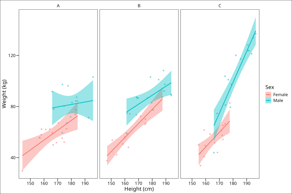

The plot shows varying relationships between height and weight across the groups and sexes. As intended by the data generation, the slope for Group C Males appears noticeably steeper than for other groups.

Fitting the Linear Model

We fit a linear model (lm) predicting Weight based on Group, Sex, and Height, including all possible interactions (Group * Sex * Height). This allows the relationship (slope) between Height and Weight to differ for every combination of Group and Sex.

model_hws <- lm(Weight ~ Group * Sex * Height, data = df_hws)
summary(model_hws)

Call:
lm(formula = Weight ~ Group * Sex * Height, data = df_hws)

Residuals:
     Min       1Q   Median       3Q      Max 
-21.1212  -6.0448   0.0515   5.6366  18.8071 

Coefficients:
                       Estimate Std. Error t value Pr(>|t|)    
(Intercept)            -69.9453    43.1485  -1.621 0.10905    
GroupB                 -50.5078    58.8345  -0.858 0.39326    
GroupC                 -66.3386    70.8607  -0.936 0.35207    
SexMale                116.8949    71.4718   1.636 0.10597    
Height                   0.7731     0.2604   2.968 0.00398 ** 
GroupB:SexMale         -34.0398    92.3319  -0.369 0.71337    
GroupC:SexMale        -317.5395   102.8442  -3.088 0.00279 ** 
GroupB:Height            0.3281     0.3558   0.922 0.35922    
GroupC:Height            0.3807     0.4277   0.890 0.37612    
SexMale:Height          -0.5803     0.4106  -1.414 0.16148    
GroupB:SexMale:Height    0.1817     0.5328   0.341 0.73394    
GroupC:SexMale:Height    1.8487     0.5938   3.113 0.00259 ** 
---
Signif. codes:  0 ‘***’ 0.001 ‘**’ 0.01 ‘*’ 0.05 ‘.’ 0.1 ‘ ’ 1

Residual standard error: 9.758 on 78 degrees of freedom
Multiple R-squared:  0.8552,	Adjusted R-squared:  0.8348 
F-statistic: 41.88 on 11 and 78 DF,  p-value: < 2.2e-16

The model summary shows significant two-way (GroupC:SexMale) and three-way (GroupC:SexMale:Height) interactions involving Group C and Males. This strongly suggests the relationship between height and weight is different for males in group C. The emtrends function provides a more direct way to test specific hypotheses about these slopes.

1. One-Sample Slope Test

Question: Do males in Group A have a significantly positive relationship (i.e., slope > 0) between height and weight?

We use emmeans::emtrends(), which fortunately behaves almost identically to its emmeans::emmeans() counterpart – specifying the model, the factors defining the groups (~ Group * Sex). The at argument filters to “Male” in “Group A”. We test against a null hypothesis of 0 (null = 0) using a one-sided test (side = "right"). Crucially, this function has one more important argument var, which is the the continuous variable for which we want to compare the slopes for. In our case, "Height".

emmeans::emtrends(
  model_hws, 
  ~ Group * Sex, 
  at = list(Group = "A", Sex = "Male"), 
  var = "Height",
  side = "right",
  null = 0
) %>%
  broom.mixed::tidy()

# A tibble: 1 × 7
  Group Sex   Height.trend std.error    df statistic p.value
  <chr> <chr>        <dbl>     <dbl> <dbl>     <dbl>   <dbl>
1 A     Male         0.193     0.317    78     0.607   0.273

The estimated slope (Height.trend) for Group A males is 0.193. The p-value of 0.273 suggests that this slope is not significantly greater than zero. We do not have sufficient evidence to conclude there is a positive relationship between height and weight for males in Group A in this dataset.

2. Two-Sample Slope Comparison

Question: Is there a difference in the relationship (slope) between height and weight for males versus females within Group C?

We first get the trends for Males and Females in Group C using emmeans::emtrends() and the at argument, then pipe to emmeans::contrast(method = "pairwise") to compare these two slopes.

# Q: Is Height-Weight slope different between Group C Males and Group C Females?
emmeans::emtrends(
  model_hws,
  ~ Group * Sex,
  at = list(Group = "C", Sex = c("Male", "Female")),
  var = "Height"
) %>%
  emmeans::contrast(
    method = "pairwise",
    adjust = "bonferroni"
  ) %>%
  broom.mixed::tidy()

# A tibble: 1 × 8
  term      contrast          null.value estimate std.error    df statistic p.value
  <chr>     <chr>                  <dbl>    <dbl>     <dbl> <dbl>     <dbl>   <dbl>
1 Group*Sex C Male - C Female          0     1.27     0.429    78      2.96 0.00411

The estimated difference in slopes (Male – Female in Group C) is 1.27. The very small p-value (0.00411) indicates a highly significant difference. As we deliberately designed for this dataset, males in Group C have a significantly steeper positive relationship between height and weight compared to females in Group C.

3. Interaction Test for Slopes

Question: Does the difference in height-weight slopes between males and females change significantly when moving from Group B to Group C?

We get the trends for both sexes in Groups B and C using emmeans::emtrends() and the at argument, then use emmeans::contrast(interaction = "pairwise"). This tests if the (Male slope – Female slope) difference is different between Group B and Group C.

# Q: Does (Male slope - Female slope) differ between Group B and Group C?
emmeans::emtrends(
  model_hws,
  ~ Group * Sex,
  at = list(Group = c("B", "C"), Sex = c("Male", "Female")),
  var = "Height"
) %>%
  emmeans::contrast(
    interaction = "pairwise",
    adjust = "bonferroni"
  ) %>%
  broom.mixed::tidy()

# A tibble: 1 × 8
  term      Group_pairwise Sex_pairwise  estimate std.error    df statistic p.value
  <chr>     <chr>          <chr>            <dbl>     <dbl> <dbl>     <dbl>   <dbl>
1 Group*Sex B - C          Male - Female    -1.67     0.547    78     -3.05 0.00315

The output shows the interaction contrast: (B Male – B Female) – (C Male – C Female). The estimate is -1.67, and the p-value (0.00315) is significant. This indicates that the way the height-weight slope differs between sexes is significantly different when comparing Group B to Group C. Specifically, the male-female slope difference is much larger in Group C than in Group B.

Connecting Back to Model Coefficients

Just like with emmeans::emmeans(), we can relate emmeans::emtrends() contrasts back to the model coefficients, although it requires careful consideration of reference levels. Let us try to replicate the GroupB:SexMale:Height coefficient (Estimate = 0.1817, p = 0.734) from the summary(model_hws) output. This coefficient represents how the slope difference between male and the reference female changes when moving from the reference Group A to Group B.

We can test this using an interaction contrast focusing on Groups A and B, and both Sexes. Note the use of interaction = "trt.vs.ctrl" which compares each factor’s levels against its reference level.

# Q: Replicate the model coefficient for GroupB:SexMale:Height interaction
# This represents (B:Male - B:Female) - (A:Male - A:Female) slope differences,
# or equivalently, (B:Male - A:Male) - (B:Female - A:Female)
emmeans::emtrends(
  model_hws,
  ~ Group * Sex,
  at = list(Group = c("A", "B"), Sex = c("Male", "Female")),
  var = "Height"
) %>%
  emmeans::contrast(
    # Compare Group B vs A (ref) within Male vs Female (ref)
    interaction = c("trt.vs.ctrl", "trt.vs.ctrl"), 
    adjust = "none" # No adjustment for single coefficient replication
  ) %>%
  broom.mixed::tidy()

# A tibble: 1 × 8
  term      Group_trt.vs.ctrl Sex_trt.vs.ctrl estimate std.error    df statistic p.value
  <chr>     <chr>             <chr>                  <dbl>     <dbl> <dbl>     <dbl>   <dbl>
1 Group*Sex B                 Male               0.182     0.533    78     0.341   0.734

The estimate (0.182) and p-value (0.734) match the GroupB:SexMale:Height coefficient in the model summary. This again highlights that emmeans::emtrends allows flexible testing of slope comparisons, including those represented by complex interaction terms in the original model summary.

Conclusion

Contrasts and post-hoc tests are indispensable tools for moving beyond the general output of statistical models to answer specific, nuanced research questions. The emmeans package in R, with its emmeans() and emtrends() functions, provides a powerful and flexible framework for conducting these detailed analyses. Whether you are comparing adjusted group means or the slopes of relationships, emmeans simplifies the process of specifying comparisons, performing tests, and obtaining clear, interpretable results, even for complex models involving interactions and random effects.

Prev Linear Mixed Effects Models (LMEs)

End of Module

Great job on working through the core statistical methods in R! You’re now equipped to test hypotheses and model data. The journey doesn’t end here, however. The next module, “Ecology and Evolutionary Biology (EEB) Analyses,” takes a deeper dive into using R and specialized third-party packages for the kinds of sophisticated analyses frequently employed in EEB. Get ready to tackle some of the cornerstone analytical techniques in the field!

Whenever you’re ready, click the link below to proceed to the next module:

EEB Analyses

R Manual Ecology &
Evolutionary Biology

Contrasts and Post-Hoc Testing

Statistics in R

Introduction

Example 1: Plant Defenses in Kluane – Using `emmeans`

Data Preparation and Visualization

Fitting the Mixed-Effects Model

Interpreting the Default Summary (and its Limitations)

Using `emmeans` for Specific Comparisons

1. One-Sample Comparisons: Testing Against a Specific Value

2. Two-Sample Comparisons: Comparing Specific Groups

The method argument

3. Interaction Contrasts: Comparing Differences of Differences

Connecting Back to Model Coefficients

Example 2: Analyzing Slopes with `emtrends`

Data Generation and Visualization

Fitting the Linear Model

1. One-Sample Slope Test

2. Two-Sample Slope Comparison

3. Interaction Test for Slopes

Connecting Back to Model Coefficients

Conclusion

End of Module

Statistics in R

Introduction

Example 1: Plant Defenses in Kluane – Using emmeans

Data Preparation and Visualization

Fitting the Mixed-Effects Model

Interpreting the Default Summary (and its Limitations)

Using emmeans for Specific Comparisons

1. One-Sample Comparisons: Testing Against a Specific Value

2. Two-Sample Comparisons: Comparing Specific Groups

The method argument

3. Interaction Contrasts: Comparing Differences of Differences

Connecting Back to Model Coefficients

Example 2: Analyzing Slopes with emtrends

Data Generation and Visualization

Fitting the Linear Model

1. One-Sample Slope Test

2. Two-Sample Slope Comparison

3. Interaction Test for Slopes

Connecting Back to Model Coefficients

Conclusion

End of Module

Example 1: Plant Defenses in Kluane – Using `emmeans`

Using `emmeans` for Specific Comparisons

Example 2: Analyzing Slopes with `emtrends`