Understanding Linear Mixed Effects Models

Before diving into the practical application, it’s essential to understand how LME models differ from traditional linear models and why they’re particularly useful in ecological research.

Hierarchical Data Structures

In ecological research, data often exhibit natural hierarchical structures. For example:

• Students within Classes within Schools within Districts
• Individuals within Populations within Species
• Repeated Measurements within Individuals within Populations

These hierarchical structures can be either nested or crossed:

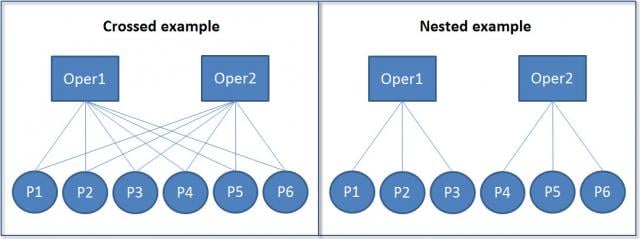
In nested structures (right), each lower-level unit belongs to only one higher-level unit. For example, each student belongs to only one class, and each class belongs to only one school. In crossed structures (left), lower-level units can belong to multiple higher-level units. For example, a student might take multiple classes, and a teacher might teach multiple classes.

Simpson’s Paradox

Simpson’s Paradox is a statistical phenomenon where a trend appears in different groups of data but disappears or reverses when the groups are combined. This is particularly relevant in ecological studies where data are often nested or grouped. Consider the following example using the Palmer Penguins dataset:

library(tidyverse)
library(palmerpenguins)
df_penguins <- penguins

# Plot
model_penguins <- lm(bill_depth_mm ~ bill_length_mm, data = df_penguins %>% drop_na())

df_penguins %>%
  drop_na() %>%
  mutate(
    predicted = predict(model_penguins)
  ) %>%
  ggplot(aes(x = bill_length_mm, y = bill_depth_mm, color = species)) +
  geom_point() +
  geom_smooth(method = "lm", se = FALSE) +
  geom_abline(
    intercept = coef(model_penguins)[1],
    slope = coef(model_penguins)[2],
    color = "black",
    size = 2
  ) +
  labs(
    title = "Demonstration of Simpson's Paradox",
    x = "Bill Length (mm)",
    y = "Bill Depth (mm)",
    color = "Species"
  ) +
  ggthemes::theme_base()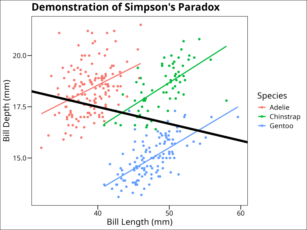

In this example, when we fit a simple linear regression to all penguins (black line), we see a positive relationship between bill length and bill depth. However, when we look at each species separately (colored lines), we see negative relationships. This apparent contradiction is Simpson’s Paradox, and it occurs because species is a confounding variable that affects both bill length and bill depth.

Whereas traditional linear models will overlook the underlying trends within data hierarchy, linear mixed effects models are designed to incorporate them.

Model Structure

A traditional linear model can be written as:

y_i = \beta_0 + \beta_1x_i + \epsilon_i

where:

• \(y_i\) is the response variable for observation i
• \(\beta_0\) is the intercept
• \(\beta_1\) is the slope coefficient
• \(x_i\) is the predictor variable
• \(\epsilon_i\) is the residual error

A linear mixed effects model extends this by adding random effects:

y_{ij} = \beta_0 + \beta_1x_{ij} + u_j + \epsilon_{ij}

where:

• \(y_{ij}\) is the response variable for observation i in group j
• \(x_{ij}\) is the predictor variable for observation i in group j
• \(u_j\) is the random effect for group j
• \(\epsilon_{ij}\) is the residual error for observation i in group j

The key difference is that the error term is now split into two components: the random effect \(u_j\) and the residual error \(\epsilon_{ij}\). This decomposition allows us to model both systematic variation (through random effects) and residual variation separately.

Advantages of Linear Mixed Effects Models

LME models offer several advantages over traditional linear models:

• Handling Nested Data: LME models naturally account for hierarchical structures in data, such as multiple measurements within individuals or sites within regions.
• Relaxed Independence Assumption: Traditional linear models assume all observations are independent. LME models allow for correlation within groups through random effects.
• Partial Pooling: LME models balance between complete pooling (treating all data as one group) and no pooling (treating each group separately). This is particularly useful when some groups have few observations.
• Flexible Error Structures: LME models can accommodate various types of correlation structures within groups, making them suitable for repeated measures and longitudinal data.

Remaining Assumptions and Limitations

While LME models are more flexible than traditional linear models, they still have important assumptions:

• Normality: Both random effects and residuals are assumed to follow normal distributions.
• Linear Relationships: The relationship between predictors and the response variable should be linear.
• Homogeneity of Variance: While LME models can handle some heteroscedasticity through random effects, they still assume constant variance within groups.
• Random Effects Structure: The random effects structure must be correctly specified. This requires careful consideration of the hierarchical structure in your data.

Limitations include:

• Computational Complexity: LME models can be computationally intensive, especially with many random effects or complex correlation structures.
• Sample Size Requirements: While LME models can handle unbalanced designs, they still require sufficient observations at each level of the hierarchy. If this requirement is not met, we will encounter overfitting, or the model will be unable to converge on a solution.
• Interpretation Challenges: The presence of both fixed and random effects can make model interpretation more complex than traditional linear models.

Example: Species Richness in Intertidal Areas

We’ll explore LME models using the RIKZ dataset, which examines species richness in intertidal areas. The data structure is hierarchical: multiple sites within each beach, with abiotic variables measured at each site.

The RIKZ dataset contains the following variables:

• Richness: The number of species found at each site
• NAP: Normal Amsterdams Peil, a measure of height relative to mean sea level
• Beach: A factor identifying each beach (1-9)
• Site: A factor identifying each site within a beach (1-5)

Data Preparation

First, let’s load and prepare our data:

library(tidyverse)
library(lme4) # for linear mixed effects models
library(lmerTest) # load in to get p-values in linear mixed effects models
library(broom.mixed) # for tidy output from linear mixed effects models

# Load the RIKZ dataset
df_rikz <- read_tsv("https://uoftcoders.github.io/rcourse/data/rikz_data.txt")

# Site and Beach are factors
df_rikz <- df_rikz %>%
  mutate(
    Site = factor(Site),
    Beach = factor(Beach)
  )
str(df_rikz)

spc_tbl_ [45 × 5] (S3: spec_tbl_df/tbl_df/tbl/data.frame)
 $ Richness: num [1:45] 11 10 13 11 10 8 9 8 19 17 ...
 $ Exposure: num [1:45] 10 10 10 10 10 8 8 8 8 8 ...
 $ NAP     : num [1:45] 0.045 -1.036 -1.336 0.616 -0.684 ...
 $ Beach   : num [1:45] 1 1 1 1 1 2 2 2 2 2 ...
 $ Site    : num [1:45] 1 2 3 4 5 1 2 3 4 5 ...

The data contains 45 observations across 9 beaches, with 5 sites per beach. We’ve encoded ‘Beach’ as a factor to facilitate its use as a random effect.

Initial Linear Regression

Let’s start with a simple linear regression to examine the relationship between species richness and NAP, pooling data across all beaches:

# Linear regression
lm_base <- lm(Richness ~ NAP, data = df_rikz)
summary(lm_base)

Call:
lm(formula = Richness ~ NAP, data = df_rikz)

Residuals:
    Min      1Q  Median      3Q     Max 
-5.0675 -2.7607 -0.8029  1.3534 13.8723 

Coefficients:
            Estimate Std. Error t value Pr(>|t|)    
(Intercept)   6.6857     0.6578  10.164 5.25e-13 ***
NAP          -2.8669     0.6307  -4.545 4.42e-05 ***
---
Signif. codes:  0 ‘***’ 0.001 ‘**’ 0.01 ‘*’ 0.05 ‘.’ 0.1 ‘ ’ 1

Residual standard error: 4.16 on 43 degrees of freedom
Multiple R-squared:  0.3245,    Adjusted R-squared:  0.3088 
F-statistic: 20.66 on 1 and 43 DF,  p-value: 4.418e-05

# Plot the data
ggplot(df_rikz, aes(x = NAP, y = Richness)) +
  geom_point() +
  geom_smooth(method = "lm", se = FALSE) +
  ggthemes::theme_base()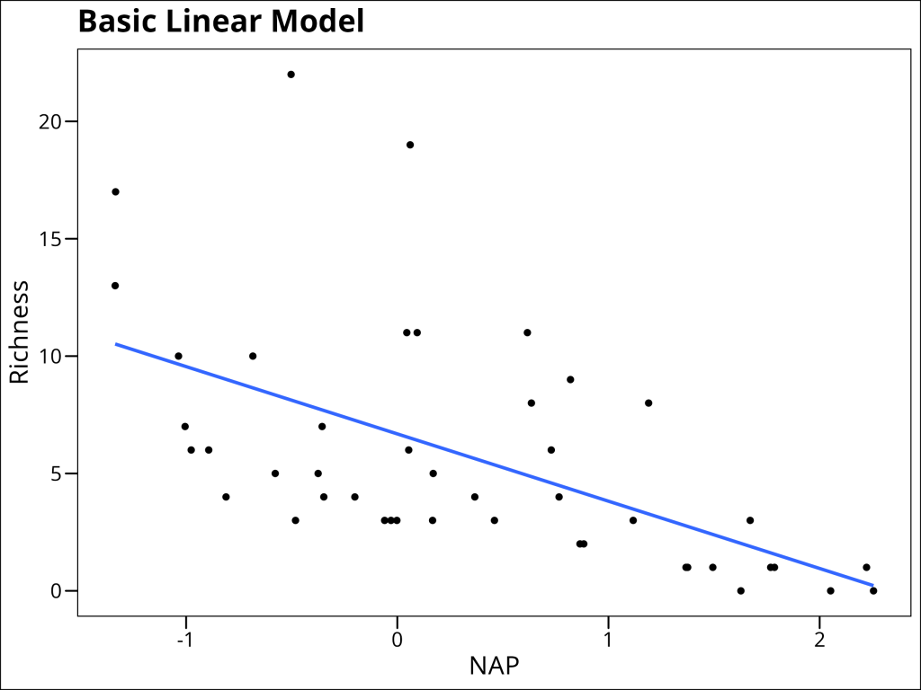

Okay, we observe a general linear decrease. But this model makes the underlying assumption that all beaches have the same relationship between the two variables. Adding covariates is just another way of saying that we are…

Adding more fixed effects

Yes, in essence, covariates in a linear model are just additional fixed effects in the model specification. In this case, we can add a fixed effect of Beach to model our belief that every beach offers a different relationship between NAP and species Richness.

lm_fixed_beach <- lm(Richness ~ NAP + Beach, data = df_rikz)
summary(lm_fixed_beach)

Call:
lm(formula = Richness ~ NAP + Beach, data = df_rikz)

Residuals:
    Min      1Q  Median      3Q     Max 
-4.8518 -1.5188 -0.1376  0.7905 11.8384 

Coefficients:
            Estimate Std. Error t value Pr(>|t|)    
(Intercept)   9.8059     1.3895   7.057 3.22e-08 ***
NAP          -2.4928     0.5023  -4.963 1.79e-05 ***
Beach2        3.0781     1.9720   1.561  0.12755    
Beach3       -6.4049     1.9503  -3.284  0.00233 ** 
Beach4       -6.0329     2.0033  -3.011  0.00480 ** 
Beach5       -0.8983     2.0105  -0.447  0.65778    
Beach6       -5.2231     1.9682  -2.654  0.01189 *  
Beach7       -5.4367     2.0506  -2.651  0.01196 *  
Beach8       -4.5530     1.9972  -2.280  0.02883 *  
Beach9       -3.7820     2.0060  -1.885  0.06770 .  
---
Signif. codes:  0 ‘***’ 0.001 ‘**’ 0.01 ‘*’ 0.05 ‘.’ 0.1 ‘ ’ 1

Residual standard error: 3.06 on 35 degrees of freedom
Multiple R-squared:  0.7025,    Adjusted R-squared:  0.626 
F-statistic: 9.183 on 9 and 35 DF,  p-value: 5.645e-07

Or, represented as a plot:

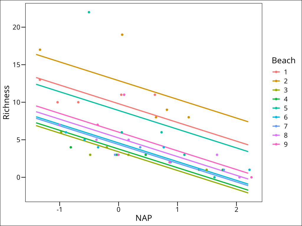
Unfortunately, a lot of degrees of freedom being lost with this approach. You might think “can’t we just fit N individual linear regressions then, one per beach?” Well, yes, but consider that every model counts as a statistical test. We must correct for the number of statistical tests we conduct and therefore we would quickly find ourselves losing statistical power on two fronts. Firstly, due to correcting for N tests and weakening our power by N times, and secondly, each model would feature fewer datapoints:

df_rikz %>%
  group_by(Beach) %>%
  summarise(n = n())

  Beach     n
  <fct> <int>
1 1         5
2 2         5
3 3         5
4 4         5
5 5         5
6 6         5
7 7         5
8 8         5
9 9         5

Can we avoid this outcome while avoiding loss of degrees of freedom?

Random Intercepts Model

Yes! By having our model respect the hierarchical nature of this data. In this case, that the data is grouped into subsets by Beach. We can therefore begin by stating that every beach is permitted to have its own intercept in the model. Aka, a random intercept.

In R’s formula notation, this is specified as:

# Random Intercepts Model
lme_randint_beach <- lmer(
  Richness ~ NAP + (1 | Beach),
  data = df_rikz,
  REML = FALSE
)

The model formula includes:

• Fixed Effects: NAP (the main predictor)

• Random Effects: (1 | Beach) specifies random intercepts for each beach
  • Beach is our grouping variable
  • The | separates the random effects from the grouping variable.
  • The 1 indicates we’re only modeling random intercepts

Let’s examine the model summary output

summary(lme_randint_beach)

Linear mixed model fit by maximum likelihood . t-tests use Satterthwaite's method ['lmerModLmerTest']
Formula: Richness ~ NAP + (1 | Beach)
   Data: df_rikz

     AIC      BIC   logLik deviance df.resid 
   249.8    257.1   -120.9    241.8       41 

Scaled residuals: 
    Min      1Q  Median      3Q     Max 
-1.4258 -0.5010 -0.1791  0.2452  4.0452 

Random effects:
 Groups   Name        Variance Std.Dev.
 Beach    (Intercept) 7.507    2.740   
 Residual             9.111    3.018   
Number of obs: 45, groups:  Beach, 9

Fixed effects:
            Estimate Std. Error      df t value Pr(>|t|)    
(Intercept)   6.5844     1.0321  9.4303   6.380 0.000104 ***
NAP          -2.5757     0.4873 38.2433  -5.285 5.34e-06 ***
---
Signif. codes:  0 ‘***’ 0.001 ‘**’ 0.01 ‘*’ 0.05 ‘.’ 0.1 ‘ ’ 1

Correlation of Fixed Effects:
    (Intr)
NAP -0.164

• Fixed Effects: Shows the estimated coefficients for NAP and the intercept, along with their standard errors and p-values
• Random Effects: Shows the variance and standard deviation of the random intercepts for Beach and the residual variance
• Number of Observations: Shows the total number of observations and the number of groups (beaches)

Let’s visualize the model’s predictions amid the current data:

df_rikz %>%
  mutate(predicted = predict(lme_randint_beach)) %>%
  ggplot(aes(x = NAP, y = Richness, color = Beach)) +
  # Add the main effect line
  geom_abline(
    intercept = fixef(lme_randint_beach)[1],
    slope = fixef(lme_randint_beach)[2],
    color = "black",
    size = 2
  ) +
  # Add the random effect lines
  geom_line(aes(y = predicted)) +
  geom_point(size = 2) +
  ggthemes::theme_base()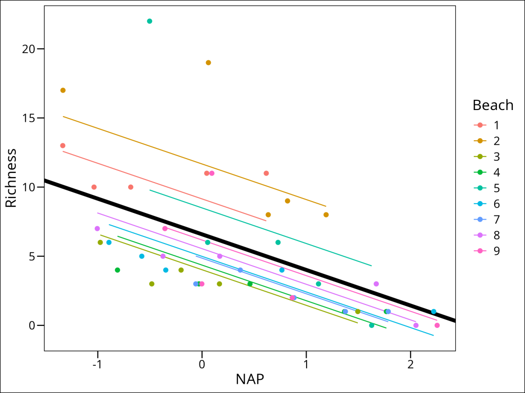

This is a step in the right direction!

However, this model still makes the assumption that the slope describing the relationship between Richness and NAP is the same for all beaches. Is this really the case? Let’s plot each beach separately to see:

ggplot(df_rikz, aes(x = NAP, y = Richness)) +
  geom_point() +
  geom_smooth(method = "lm", se = FALSE) +
  facet_wrap(~Beach) +
  ggthemes::theme_base() +
  ggsave("src/Statistics_in_R/images/fig_lme_beach_facet.png",
    last_plot(),
    width = 8, height = 6
  )

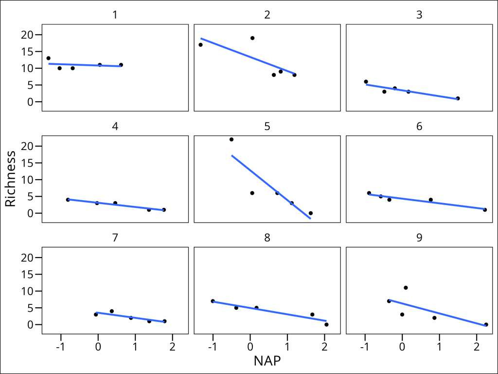
Indeed, it appears that the relationship differs drastically for certain beaches (i.e. compare Beach 1 with Beach 5). This can be solved by going one step further by introducing random slopes to our model.

Random Intercepts and Slopes Model

We can extend our model to include random slopes, allowing the relationship between NAP and species richness to vary by beach. In R’s formula notation, this is specified as:

# Random Intercepts and Slopes Model
lme_randint_slope_beach <- lmer(Richness ~ NAP + (NAP | Beach), data = df_rikz, REML = FALSE)
summary(lme_randint_slope_beach)

Linear mixed model fit by maximum likelihood . t-tests use Satterthwaite's method ['lmerModLmerTest']
Formula: Richness ~ NAP + (NAP | Beach)
   Data: df_rikz

     AIC      BIC   logLik deviance df.resid 
   246.7    257.5   -117.3    234.7       39 

Scaled residuals: 
    Min      1Q  Median      3Q     Max 
-1.7985 -0.3418 -0.1827  0.1749  3.1389 

Random effects:
 Groups   Name        Variance Std.Dev. Corr 
 Beach    (Intercept) 10.949   3.309         
          NAP          2.502   1.582    -1.00
 Residual              7.174   2.678         
Number of obs: 45, groups:  Beach, 9

Fixed effects:
            Estimate Std. Error      df t value Pr(>|t|)    
(Intercept)   6.5818     1.1883  8.8936   5.539 0.000377 ***
NAP          -2.8293     0.6849  7.9217  -4.131 0.003366 ** 
---
Signif. codes:  0 ‘***’ 0.001 ‘**’ 0.01 ‘*’ 0.05 ‘.’ 0.1 ‘ ’ 1

Correlation of Fixed Effects:
    (Intr)
NAP -0.810
optimizer (nloptwrap) convergence code: 0 (OK)
boundary (singular) fit: see help('isSingular')

The model formula now includes:

• Fixed Effects: NAP (the main predictor)
• Random Effects: (NAP | Beach) specifies both random intercepts and slopes for NAP by Beach
  • NAP before the | indicates we’re modeling random slopes for NAP.
  • As in regular models, the 1 representing the intercept is implied and not written out. 0 + NAP would be necessary to specify only the random slopes without a random intercept for this grouping variable.
  • The | separates the random effects from the grouping variable
  • Beach is our grouping variable

Note the warning message: “boundary (singular) fit: see help(‘isSingular’)”.

This occurs when the model is overfitted or when there’s not enough variation in the data to estimate all the random effects. In this case, it suggests that the random slopes & intercepts model might be too complex for our data.

Some observations:

• With only 9 beaches, we don’t have enough groups to reliably estimate the variance-covariance structure of random slopes
• The perfect negative correlation (-1.00) between random intercepts and slopes suggests the model is overfitted

Normally, we would stop here. But for the sake of completion, let’s visualize this more complex overfit model:

df_rikz %>%
  mutate(predicted = predict(lme_randint_slope_beach)) %>%
  ggplot(aes(x = NAP, y = Richness, color = Beach)) +
  geom_abline(
    aes(
      intercept = fixef(lme_randint_slope_beach)[1],
      slope = fixef(lme_randint_slope_beach)[2]
    ),
    color = "black", size = 2
  ) +
  geom_line(aes(y = predicted)) +
  geom_point(size = 2) +
  ggthemes::theme_base()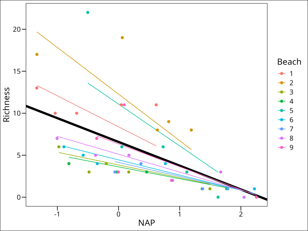

This is, unfortunately, the typical downside one encounters with mixed effects models: the tendency to over-fit. The following are rules of thumb to follow in avoiding this outcome:

• Each grouping variable should have 10+ levels
• Each random effect for a grouping variable should have 5+ datapoints within it, multiplied by the number random effects for that grouping variable. In this case, having 5 datapoints per beach is not sufficient to model both a random intercept and a random slope per beach. We should collect more data until approximately 10 datapoints are available per beach on average.

Nested Random Effects

While our data structure shows sites nested within beaches, we don’t have enough observations to properly model this hierarchy. With only 5 sites per beach, we don’t have sufficient data to estimate the variance components for both levels of nesting reliably. However, it’s worth noting the formula notation for nested random effects:

# Nested Random Effects Model
lme_nested <- lmer(Richness ~ NAP + (1 | Beach/Site), data = df_rikz, REML = FALSE)
summary(lme_nested)

The formula notation (1 | Beach/Site) represents:

• Fixed Effects: NAP (the main predictor)
• Random Effects: (1 | Beach/Site) specifies random intercepts for both Beach and Site nested within Beach
  • The / operator indicates nesting
  • This is equivalent to (1 | Beach) + (1 | Beach:Site)

In this case, with only 5 sites per beach, we don’t have enough observations to reliably estimate the variance components for both levels of nesting. This is a common limitation in ecological studies where logistical constraints limit the number of observations at each level of the hierarchy. For proper nested random effects modeling, we would typically want at least 10-15 observations per level of nesting.

Model Comparison and Selection

When comparing mixed effects models, it’s important to note that we cannot directly compare them to traditional linear models. This is because:

• Mixed effects models and linear models use different estimation methods
• The likelihood functions are not directly comparable
• The assumptions about the error structure differ fundamentally

Instead, we should compare different mixed effects models to each other and each should be fully fitted (i.e. no convergence or singularity warnings or errors).

Note that for demonstration purposes only, we will ignore the latter warning. As in previous sections, models can be compared using the anova function:

# Compare using likelihood ratio test
anova(lme_randint_beach, lme_randint_slope_beach)

Models:
lme_randint_beach: Richness ~ NAP + (1 | Beach)
lme_randint_slope_beach: Richness ~ NAP + (NAP | Beach)
                        npar    AIC    BIC  logLik deviance Chisq Df Pr(>Chisq)  
lme_randint_beach          4 249.83 257.06 -120.92   241.83                      
lme_randint_slope_beach    6 246.66 257.50 -117.33   234.66 7.173  2    0.02769 *
---
Signif. codes:  0 ‘***’ 0.001 ‘**’ 0.01 ‘*’ 0.05 ‘.’ 0.1 ‘ ’ 1

This example clearly shows the dangers of ignoring warnings in the previous steps and going down a false sense of statistical security. While the random slopes & intercepts model is demonstrated to be “better” in terms of AIC, BIC, and deviance, we know from earlier that the model overfits the data and is not valid. Proceeding with such a model would be erroneous at best.

Again, it is important NOT TO IGNORE warnings as these models are fit.

Conclusion

Linear Mixed Effects models provide a powerful framework for analyzing hierarchical data structures common in ecological research. By properly accounting for nested relationships and group-level variation, these models can:

• Handle non-independence of observations
• Model both fixed and random effects
• Provide more accurate parameter estimates
• Allow for flexible modeling of group-level variation

Understanding and properly applying LME models is crucial for ecological research where data often exhibit natural hierarchical structures.