Linear Regression

What factors influence bison mass in a restored ecosystem?

One of the first chapters to a book on causal inference that I have recently read is entitled “All you need is regression”. I thought this was an accurate way to start this section, because that statement is true! While we cannot cover all the theory of linear regression here, it is genuinely the case that nearly all classical frequentist statistical methods are simply a version of linear regression. A t-test? Actually just linear regression. ANOVA? Yup, also linear regression. Machine learning?? Many types of it are in fact just regression!

So why then, you may ask, did we learn about t-tests before we learned about linear regression in stats class? Well, it turns out that as with almost all quantitative methods discussed in this section, linear regression is frightfully easy to implement, but actually not so simple “under the hood.”

However, getting an intuitive understanding of the basics is very much possible and highly encouraged. Linear regression is probably the most fundamental of all topics you may learn in statistics, and it’s worth thinking about it carefully. To be clear, you will likely re-visit this topic many times, likely over the course of years, adding and refreshing pieces of information that will eventually develop into a solid understanding. Here, we attempt only to provide a brief introduction to the basics.

A gross simplification of the process of linear regression would be that if we want to predict the value of one continuous variable from another, we want to find a straight line that goes through as many of those points as possible.

What does it mean to do such a thing? Well, let’s start with reminding ourselves, mathematically, what a line is. A straight line is defined by the equation

y = mx + b

where $b$ is the y-intercept, $m$ is the slope of the line, and $x$ and $y$ are data values. This means that given a point on the x-axis, $x$, a slope $m$, and a y-intercept $b$, we can find the value $y$ that denotes the y-axis value that corresponds to the x-axis value $x$.

When we talk about linear regression, we’ll probably want to discuss this equation in a slightly altered form:

\widehat{weight} = \beta_0 + \beta_1 \cdot \text{is\_Male}

We’ll discuss what these terms mean in a moment but they relate exactly to a y-intercept ($\beta_0$), a slope ($\beta_1$) and an x-value.

Ordinary Least Squares (OLS)

We mentioned above we’re putting a line through some points as best we can. But how do we define this “best as we can”? Well, the version of “as best we can” that will be addressed here is the method of least squares. If we imagine a scatter of plots like this:

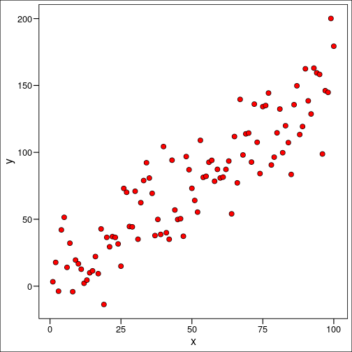
It’s clear that we can’t actually make our line go directly through very many of them, but perhaps we can figure out some way to make the line as close to as many points as possible. We’ll do that by imagining we draw a line at random, and calculate the distance between every single point and the line itself. These are called residuals. Then we’ll square each one, and take the sum of all those squares.

You might ask, why square it? The short answer to that question is that squaring it makes a large number of mathematical tools available to us. It turns out we don’t really care about the sign of the residual, that is if it’s positive or negative in relation to the regression line, just the magnitude itself.

It now follows somewhat logically that we want to find a value for the slope of our line, $\beta_1$ that minimizes this sum of the squared residuals. What we are doing here is actually a process called estimation wherein we choose some method that allows us to compare candidate values for $\beta_1$ with other values. Ordinary Least Squares is actually just a specific version of Maximum Likelihood Estimation, which we’ll discuss below.

The Linear Model

As in our previous work, we will certainly NOT (!!) just jump into writing code, as that’s the best way to ensure a poorly done analysis. First, we have our question. Let’s frame it as a hypothesis. It seems logical here to state that we think temperature will positively vary with ice cover. So a null hypothesis may be that there is no relationship between air temperature and ice cover . We have decided we want to use linear regression to tackle this challenge, so consider the assumptions of the method:

Linearity – we assume the relationship between our two variables, $X$ and $Y$ is linear
Homoscedasticity – we assume the variance of the residual is the same for any value of $X$
Normality – we assume that for any fixed value of $X$, the errors of $Y$ normally distributed
Randomness – we also assume that samples were collected at random
Independence – we assume all errors are independent

If assumptions 1-3 are violated, then we may be able to use some sort of transformation on our response variable to deal with the problem.

Let’s now get our hands dirty with a bit of an example, a very small one, that we’ll go all the way through and then delve into some details in the next example. Very generally, we can think of the process of doing regression as falling into a few steps:

Inspect our data
Perform the regression
Assess our assumptions (post-hoc)
Inspect our results
Interpret & Visualize

Here are the data we will start with:

set.seed(1234)

# Generate data
m <- 1.3 # slope
b <- 10 # intercept
sd <- 23 # standard deviation of the error term
df_simple_regression <- data.frame(
  x = seq(1, 100, 1),
  y = seq(1, 100, 1) * m + b + rnorm(100, mean = 0, sd = sd)
)
head(df_simple_regression)

  x         y
1 1 20.834041
2 2  1.681475
3 3 15.417850
4 4  3.643011
5 5 -2.497968
6 6 21.640753

Often it’s true when doing regression modelling that it’s easier to do our diagnostics of assumptions after we actually fit the model itself as some more simple tools will become available to us. So, let’s start with fitting the model. As we mentioned before, R makes it dead simple to do a linear regression in R with the lm() function.

mod_simple_regression <- lm(y ~ x, data = df_simple_regression)

That’s it! Now let’s begin seeing if what our model did was “correct”. First, we assumed linearly. We can double check this with a simple scatter plot:

df_simple_regression %>%
  ggplot(aes(x = x, y = y)) +
  geom_point(
    fill = "red", colour = "black", shape = 21,
    size = 3
  ) +
  geom_smooth(method = "lm", se = FALSE, color = "black") +
  labs(
    x = "Predictor Variable (x)",
    y = "Response Variable (y)"
  ) +
  ggthemes::theme_base()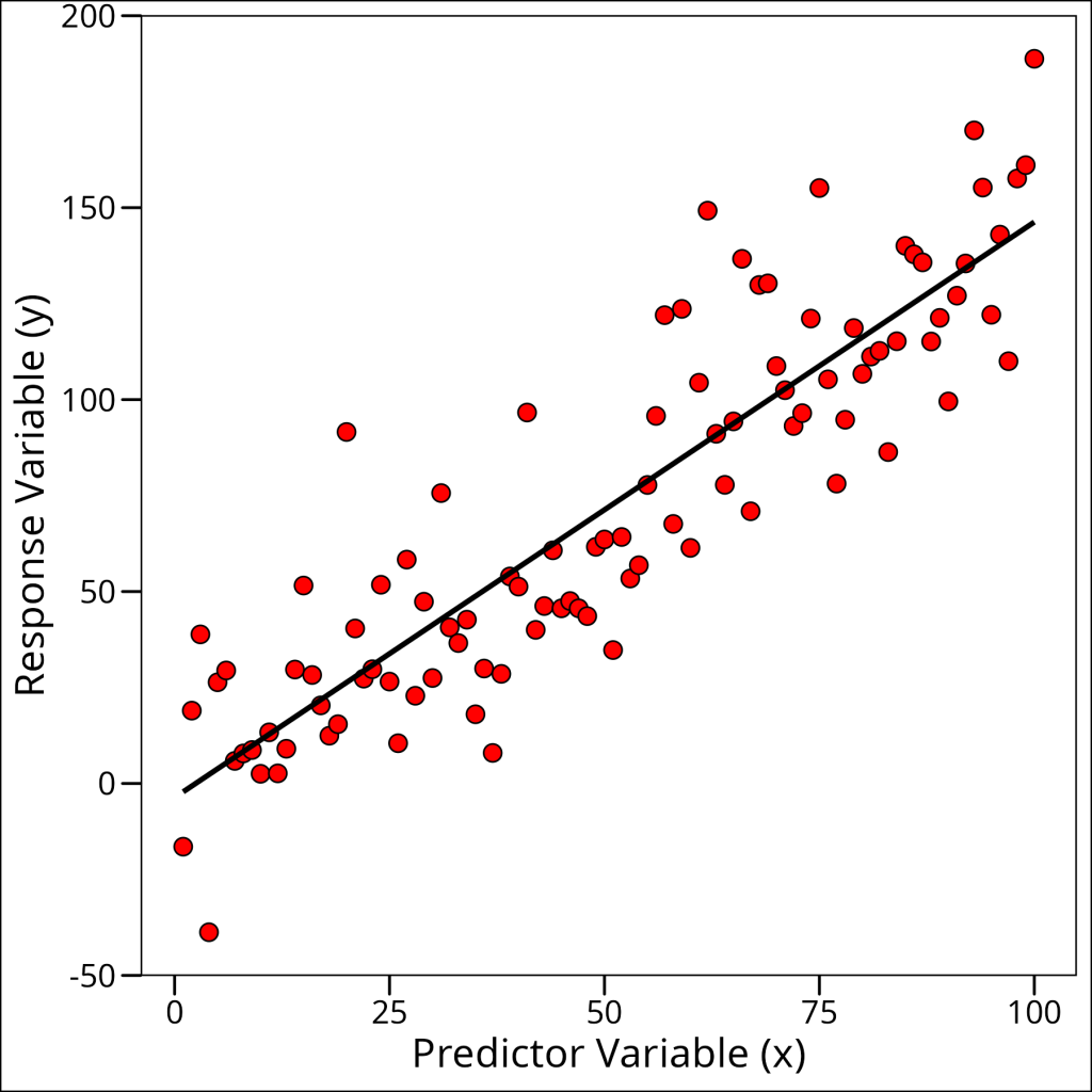

This looks sufficiently linear for our purposes. However, we can actually check all of our assumptions visually at once by using the diagnostic plots that are created by simply plotting our model object:

par(mfrow = c(2, 2))
plot(mod_simple_regression)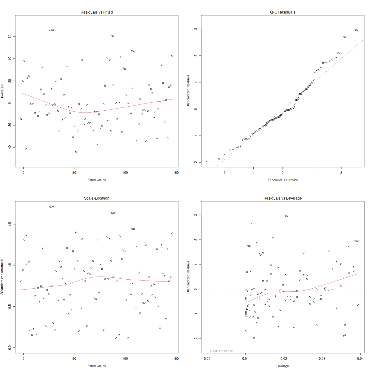

So we have four plots here.

Residuals vs. Fitted: This allows us to check the linear relationship assumption. If the red line approximately follows the grey dashed line and there are no distinct patterns, then the variables are linearly related.
Normal QQ: We interpret this the same way we interpreted QQ plots previously. If the points follow the line and don’t deviate significantly, then the residuals are normally distributed.
Spread-Location: Tests the homogeneity of variance in the residuals (our homoscedasticity). Again, we want to see a horizontal red line with “shotgun” (aka randomly spread) points.
Residuals vs. Leverage: We don’t need to look at this plot too carefully right now, but in brief, it’s used to identify points having too strong of an influence on the outcome of the analysis.

Okay so it looks like all our assumptions are satisfied! Let’s take a look at our results:

summary(mod_simple_regression)

Call:
lm(formula = y ~ x, data = df_simple_regression)

Residuals:
    Min      1Q  Median      3Q     Max
-68.109 -14.538   0.181  13.119  68.079

Coefficients:
            Estimate Std. Error t value Pr(>|t|)
(Intercept)  9.15046    4.80369   1.905   0.0597 .
x            1.33561    0.08258  16.173   <2e-16 ***
---
Signif. codes:  0 ‘***’ 0.001 ‘**’ 0.01 ‘*’ 0.05 ‘.’ 0.1 ‘ ’ 1

Residual standard error: 23.84 on 98 degrees of freedom
Multiple R-squared:  0.7274,    Adjusted R-squared:  0.7247
F-statistic: 261.6 on 1 and 98 DF,  p-value: < 2.2e-16

Let’s break down each of the components here:

1. Call — this is the function we used in our model. So to recall, what we’re showing here is the that we’ve regressed y ~ x which we would say as “y regressed against x” or “y regressed with x”.

2. Residuals — These are the residuals. Recall that a residual is the distance from a single point to the regression line at the same x-location. Here’s a visual of that:

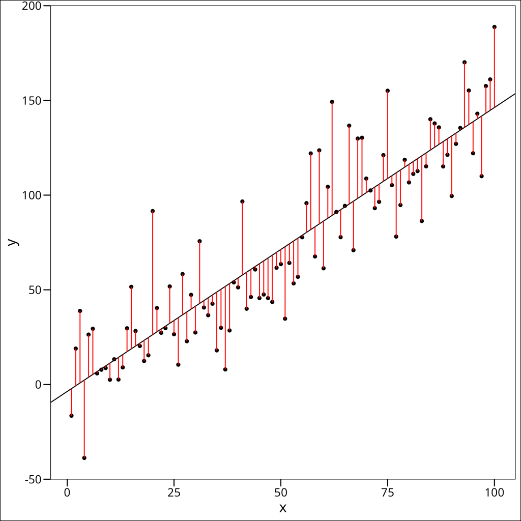
Each of the red lines here going from the points to the regression line itself are “residuals”, or “residual error”, the amount of “error” the linear model produces in its prediction for a given x-value.

The residuals here, by definition, have a mean of zero, and a “perfectly” minimized set of residuals would mean that the median value is zero, which will not really happen, but we want the median to be as close to zero as possible. We also want our minimum and maximum values to be approximately equal in magnitude.

Ok back to our summary() call.

3. Coefficients — Possibly the part that we’ll look at the most, these values are here shown as representing $\beta_0$ and $\beta_1$. So the intercept is the actual y-intercept (remember that $\beta_0$ is the y-intercept), and the $\beta_1$ is the estimate of the coefficient on $x$. We assess whether or not a particular predictor variable is significantly associated with the outcome variable via the “Pr(>|t|)” statement of the p-value. For our purposes, this will be useful, but I encourage you to interpret these p-values with caution, especially when there are multiple variables.

For our consideration, we take the Estimate as the actual estimated value for the $\beta$s and then the standard errors (SE), which quantify the uncertainty of the beta coefficient estimates. A larger SE indicates a less certain beta estimate. We then see the t-statistic and the associated p-value, which speak to the statistical significance of the beta coefficients.

We have to recall that for our regression, we are using the $H_0$ that the estimate is zero, which denotes no effect from said coefficient. If any coefficient has a p-value < 0.05, we can infer that the estimate is significantly different from zero. However, this says nothing about the strength of that relationship.

If we cared to construct a confidence interval around our beta values, we could do so with $\beta +/- 1.96 * SE_{\beta}$, which would give us our 95% CI.

4. Model Accuracy — We see a number of measures at the bottom, starting with the Residual Standard Error, which contain information about how well our model fits the data.

Starting with the Residual Standard Error (RSE), which essentially represents the average variation of the data points from the fitted regression line. It stands to reason that we want this value to be as small as possible. It comes in handy most when comparing multiple models. Say, for example, we had some other variable $z$ that we think may explain $y$, we could compare the two models $y ~ x$ and $y ~ z$ and see which model has a smaller RSE. This is not the best way to compare models, but it’s a good start.

We then see two measures of $R^2$, which is a measure of how well the model fits the data. Specifically, the measure gives the proportion of information (i.e. variation) in the data that can be explained by the model. In general, it’s preferred to use the “Adjusted R-squared” as when we add more predictors into our model, the calculation of the Adjusted R-squared will account for that.

We also see the F-statistic. The F-statistic and its associated p-value test the overall significance of the model. A large F-statistic (and a small p-value, typically < 0.05) suggests that at least one predictor variable is significantly related to the response variable. In simple linear regression with one predictor, this tests if our predictor variable (x) significantly helps explain the response variable (y).

Okay so we have all this output. What do we do with it?? Well, that depends on how we’ve formulated our hypothesis, but let’s say that we’ve stated our hypothesis to be that we think there’s a significantly non-zero relationship between x and y. Well we already have our answer in this case! If we look back at our summary() table, then we can see that our t-statistic and p-value are already given. We can see we have a significant result, which says we can reject the null hypothesis that there was no relationship (i.e. $\beta_x = 0$).

Categorical Predictor Variables

Let’s move to a real ecological example: How does adult size differ between male and female bison?

This is a good question to introduce the idea of categorical variables in a linear regression. We’ll use some data here on bison sizes, and we’re curious to estimate how much bigger males are than females. This is a categorical variable! We’re no longer regressing just one continuous variable against another. Ok first, let’s do some data manipulation.

Data Preparation

We are dealing with data on bison from the herd at Konza Prairie Biological Station LTER (KPBS) in Kansas. We happen to just be interested in adult bison, but there’s not a measure for that, so we’ll make one. A quick Google search tells us bison become sexually mature at 2-3 years of age, so we’ll filter our data so that we only keep animals older than 4, to make sure we’re comparing grown adults who’ve finished adolescence.

library(lterdatasampler)

# load in the df_bison data
df_bison <- lterdatasampler::knz_bison

# make an age variable, and filter it
df_bison <- df_bison %>%
  mutate(age = rec_year - animal_yob) %>%
  filter(age > 4) %>%
  # Ensure animal_sex is a factor for consistent modeling
  mutate(animal_sex = as.factor(animal_sex))

str(df_bison)

tibble [2,370 × 9] (S3: tbl_df/tbl/data.frame)
 $ data_code    : chr [1:2370] "CBH01" "CBH01" "CBH01" "CBH01" ...
 $ rec_year     : num [1:2370] 1994 1994 1994 1994 1994 ...
 $ rec_month    : num [1:2370] 11 11 11 11 11 11 11 11 11 11 ...
 $ rec_day      : num [1:2370] 8 8 8 8 8 8 8 8 8 8 ...
 $ animal_code  : chr [1:2370] "813" "834" "B-301" "B-402" ...
 $ animal_sex   : Factor w/ 2 levels "F","M": 1 1 1 1 1 1 1 1 1 1 ...
 $ animal_weight: num [1:2370] 890 1074 1060 989 1062 ...
 $ animal_yob   : num [1:2370] 1981 1983 1983 1984 1984 ...
 $ age          : num [1:2370] 13 11 11 10 10 9 9 9 8 8 ...

Since we will be assessing animal sex as the categorical variable of interest, let’s take a look at each level of the sex factor with a boxplot:

df_bison %>%
  ggplot(aes(x = animal_sex, y = animal_weight, fill = animal_sex)) +
  geom_boxplot() +
  labs(
    x = "Sex",
    y = "Weight (kg)",
    fill = "Sex"
  ) +
  ggthemes::theme_base()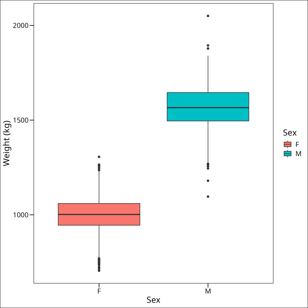

Great, these boxplots give us a visual comparison of the weight distributions for male and female bison, showing medians, spreads, and potential outliers for each group. It suggests that we have normal distributions for both groups, and that the variances are similar.

Model Fitting

So now let’s fit our model, and talk about the assumptions and the output.

mod_bison_sex <- lm(animal_weight ~ animal_sex, data = df_bison)

We’ll do some diagnostics first:

par(mfrow = c(2,2)) # this ensures all the plots show up at once
plot(mod_bison_sex)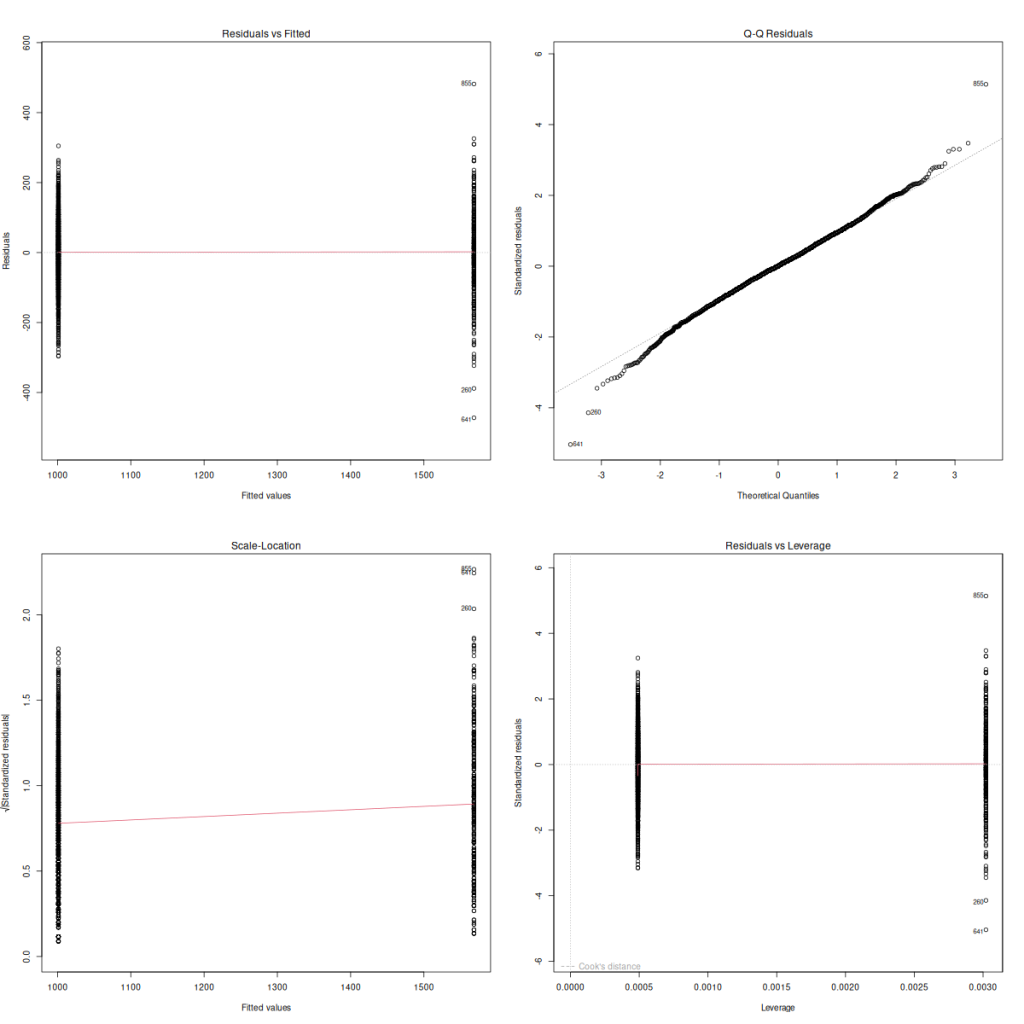

Our linearity assumption is tested by our first plot, the Residuals vs. Fitted plot, and our goal is to have a straight red line, which we do. Additionally, we can check out homoskedasticity with this plot, or with the third Scale-Location plot. We want to see an equivalent vertical spread of the points between the two groups, which we roughly do, though we can see the right side is slightly more spread out than the left, but not enough to cause us trouble. The normality of residuals we can see here in our second plot, the QQ plot. We want the points to fall along the line, with few deviations. This plot looks great. Those are our three big ones taken care of, and randomness and independence we assume from the sampling procedure.

Interpreting Results

Ok, so the important part. Interpretation. Before we even look at the output let’s think about this mathematically. Our regression equation here we can think of as this:

\widehat{weight} = \beta_0 + \beta_1 \cdot is\_Male

(Note here that we’re using the hat on top of “weight” to indicate it’s a predicted not measured value.) So recall that $\beta_0$ is the intercept, so if we find that, and we estimate our $\beta_1$ through regression, we should be able to predict the weight for any new bison that joins the herd, by taking $\beta_0$ and adding $\beta_1$ multiplied by the sex of the new bison.

But wait. How would we multiply a value “male” or “female”. Well, the thing is we can’t, and we don’t have to! Instead, R uses indicator variables (also known as dummy variables). For a categorical variable like animal_sex with levels “F” and “M”, R typically picks one level as the “reference” category (by default, the first alphabetically, so “F” in this case). It then creates an indicator variable for the other level(s). In our model summary, we see a coefficient for animal_sexM. This means R has created an internal indicator variable, let’s call it is_Male, which is:

is\_Male = \begin{cases} 1 &\text{if } animal\_sex \text{ is M} \\ 0 &\text{if } animal\_sex \text{ is F}\end{cases}

Our regression equation then effectively becomes:

\widehat{weight} = \beta_0 + \beta_1 \cdot is\_Male

Here, $\beta_0$ (the intercept in the R output) will represent the average weight for the reference category (Females), and $\beta_1$ (the coefficient for animal_sexM in the R output) will represent the difference in average weight for Males compared to Females.

Now that we’ve walked through this, let’s look at the summary and discuss.

summary(mod_bison_sex)

Call:
lm(formula = animal_weight ~ animal_sex, data = df_bison)

Residuals:
    Min      1Q  Median      3Q     Max 
-472.30  -59.25    0.75   60.75  481.70 

Coefficients:
            Estimate Std. Error t value Pr(>|t|)    
(Intercept) 1001.253      2.080   481.5   <2e-16 ***
animal_sexM  567.046      5.564   101.9   <2e-16 ***
---
Signif. codes:  0 '***' 0.001 '**' 0.01 '*' 0.05 '.' 0.1 ' ' 1

Residual standard error: 93.9 on 2368 degrees of freedom
Multiple R-squared:  0.8143,	Adjusted R-squared:  0.8142 
F-statistic: 1.038e+04 on 1 and 2368 DF,  p-value: < 2.2e-16

Let’s break down each of the components here:

2. Residuals — These are the residuals. Recall that a residual is the distance from a single point to the regression line at the same x-location. Here’s a visual of that:

Ok back to our summary() call.

If we cared to construct a confidence interval around our beta values, we could do so with $\beta +/- 1.96 * SE_{\beta}$, which would give us our 95% CI.

4. Model Accuracy — We see a number of measures at the bottom, starting with the Residual Standard Error, which contain information about how well our model fits the data.

Multiple Regression

The process of adding more variables as possible predictors is a simple one technically, but requires that we think more carefully about the model output. In this case the principle of Occam’s Razor or the law of parsimony applies, wherein, it is generally true that we are looking for the most parsimonious solution. That is, we want to identify a model which provides us the most explanatory power with respect to the data, while minimizing the number of features. So, when performing modeling exercises routed in rigorous hypothesis testing, we never add extraneous variables we don’t have a good reason to add. And we always attempt to only keep variables in the model which sufficiently add explanatory power. A linear regression with multiple predictor variables is often called multiple regression.

Let’s use an example. We’ve already used the bison example above, so let’s stick with that. Say that we hypothesized males are bigger than females (a reasonable assumption), but also that the size of individuals over all has gone down through time. While this specific herd is managed and protected, this type of hypothesis may make sense if considering a harvested population, as often hunting removes the largest individuals from a population. We fit our model above and could have determined that indeed males are larger than females in a meaningful sense. Perhaps we now wanted to understand if adding time to our model improved the “fit”. That is, if more variation in the data are explained by adding this additional parameter.

Let’s try it! So we are now using a slightly altered equation, since we’ll treat time as continuous, our model equation for a predicted weight of an individual will look like:

\widehat{weight} = \beta_0 + \beta_1 \cdot \text{is\_Male} + \beta_2 \cdot \text{year}

We may hypothesize that $\beta_2$ will be significantly lower than zero, indicating that as time increases, the effect on predicted weight will be that of a decreased weight

We want the rec_year variable, so let’s look at the spread of those data (i.e. how many years are represented):

summary(df_bison$rec_year)

   Min. 1st Qu.  Median    Mean 3rd Qu.    Max. 
   1994    2003    2009    2009    2015    2020

Okay, so we have 15 years of data. Let’s move on to the model:

mod_bison_mr <- lm(animal_weight ~ animal_sex + rec_year,
        data = df_bison)

And we’ll do our diagnostic plotting:

par(mfrow = c(2,2)) # this ensures all the plots show up at once
plot(mod_bison_mr)

These look sufficiently satisfactory. Now for the output:

summary(mod_bison_mr)

## 
Call:
lm(formula = animal_weight ~ animal_sex + rec_year, data = df_bison)

Residuals:
    Min      1Q  Median      3Q     Max 
-467.07  -59.60    0.40   59.43  484.98 

Coefficients:
             Estimate Std. Error t value Pr(>|t|)    
(Intercept) -957.0540   525.8407  -1.820 0.068878 .  
animal_sexM  566.5127     5.5512 102.051  <2e-16 ***
rec_year       0.9749     0.2618   3.724 0.000201 ***
---
Signif. codes:  0 '***' 0.001 '**' 0.01 '*' 0.05 '.' 0.1 ' ' 1

Residual standard error: 93.65 on 2367 degrees of freedom
Multiple R-squared:  0.8154,	Adjusted R-squared:  0.8152 
F-statistic:  5227 on 2 and 2367 DF,  p-value: < 2.2e-16

Okay! So it looks as though we might have been wrong! It appears as though the size of animals may be increasing through time. Technically we’ve been given a significant p-value on the coefficient of rec_year but the estimate isn’t high.

Model Objects & Subsetting

This is a good opportunity to discuss the actual object we create when we fit a linear model. We know we can call summary on our model object, but there are many other things we can do with it too.

It’s good to know first what structure the model object is:

str(mod_bison_mr)

## List of 13
##  $ coefficients : Named num [1:3] -957.054 566.513 0.975
##   ..- attr(*, "names")= chr [1:3] "(Intercept)" "animal_sexM" "rec_year"
##  $ residuals    : Named num [1:2370] -96.8 87.2 73.2 2.2 75.2 ...
##   ..- attr(*, "names")= chr [1:2370] "1" "2" "3" "4" ...
##  $ effects      : Named num [1:2370] -5.26e+04 9.57e+03 3.49e+02 5.46e-01 7.35e+01 ...
##   ..- attr(*, "names")= chr [1:2370] "(Intercept)" "animal_sexM" "rec_year" "" ...
##  $ rank         : int 3
##  $ fitted.values: Named num [1:2370] 987 987 987 987 987 ...
##   ..- attr(*, "names")= chr [1:2370] "1" "2" "3" "4" ...
##  $ assign       : int [1:3] 0 1 2
##  $ qr           :List of 5
##   ..$ qr   : num [1:2370, 1:3] -48.6826 0.0205 0.0205 0.0205 0.0205 ...
##   .. ..- attr(*, "dimnames")=List of 2
##   .. .. ..$ : chr [1:2370] "1" "2" "3" "4" ...
##   .. .. ..$ : chr [1:3] "(Intercept)" "animal_sexM" "rec_year"
##   .. ..- attr(*, "assign")= int [1:3] 0 1 2
##   .. ..- attr(*, "contrasts")=List of 1
##   .. .. ..$ animal_sex: chr "contr.treatment"
##   ..$ qraux: num [1:3] 1.02 1.01 1.04
##   ..$ pivot: int [1:3] 1 2 3
##   ..$ tol  : num 1e-07
##   ..$ rank : int 3
##   ..- attr(*, "class")= chr "qr"
##  $ df.residual  : int 2367
##  $ contrasts    :List of 1
##   ..$ animal_sex: chr "contr.treatment"
##  $ xlevels      :List of 1
##   ..$ animal_sex: chr [1:2] "F" "M"
##  $ call         : language lm(formula = animal_weight ~ animal_sex + rec_year, data = df_bison)
##  $ terms        :Classes 'terms', 'formula'  language animal_weight ~ animal_sex + rec_year
##   .. ..- attr(*, "variables")= language list(animal_weight, animal_sex, rec_year)
##   .. ..- attr(*, "factors")= int [1:3, 1:2] 0 1 0 0 0 1
##   .. .. ..- attr(*, "dimnames")=List of 2
##   .. .. .. ..$ : chr [1:3] "animal_weight" "animal_sex" "rec_year"
##   .. .. .. ..$ : chr [1:2] "animal_sex" "rec_year"
##   .. ..- attr(*, "term.labels")= chr [1:2] "animal_sex" "rec_year"
##   .. ..- attr(*, "order")= int [1:2] 1 1
##   .. ..- attr(*, "intercept")= int 1
##   .. ..- attr(*, "response")= int 1
##   .. ..- attr(*, ".Environment")= 
##   .. ..- attr(*, "predvars")= language list(animal_weight, animal_sex, rec_year)
##   .. ..- attr(*, "dataClasses")= Named chr [1:3] "numeric" "factor" "numeric"
##   .. .. ..- attr(*, "names")= chr [1:3] "animal_weight" "animal_sex" "rec_year"
##  $ model        :'data.frame':	2370 obs. of  3 variables:
##   ..$ animal_weight: num [1:2370] 890 1074 1060 989 1062 ...
##   ..$ animal_sex   : Factor w/ 2 levels "F","M": 1 1 1 1 1 1 1 1 1 1 ...
##   ..$ rec_year     : num [1:2370] 1994 1994 1994 1994 1994 ...
##   ..- attr(*, "terms")=Classes 'terms', 'formula'  language animal_weight ~ animal_sex + rec_year
##   .. .. ..- attr(*, "variables")= language list(animal_weight, animal_sex, rec_year)
##   .. .. ..- attr(*, "factors")= int [1:3, 1:2] 0 1 0 0 0 1
##   .. .. .. ..- attr(*, "dimnames")=List of 2
##   .. .. .. .. ..$ : chr [1:3] "animal_weight" "animal_sex" "rec_year"
##   .. .. .. .. ..$ : chr [1:2] "animal_sex" "rec_year"
##   .. .. ..- attr(*, "term.labels")= chr [1:2] "animal_sex" "rec_year"
##   .. .. ..- attr(*, "order")= int [1:2] 1 1
##   .. .. ..- attr(*, "intercept")= int 1
##   .. .. ..- attr(*, "response")= int 1
##   .. .. ..- attr(*, ".Environment")= 
##   .. .. ..- attr(*, "predvars")= language list(animal_weight, animal_sex, rec_year)
##   .. .. ..- attr(*, "dataClasses")= Named chr [1:3] "numeric" "factor" "numeric"
##   .. .. .. ..- attr(*, "names")= chr [1:3] "animal_weight" "animal_sex" "rec_year"
##  - attr(*, "class")= chr "lm"

This is a long set of things, and we’ll not go through it all, but know first that any subset that has a $ before it is accessible as such. For example:

mod_bison_mr$coefficients

(Intercept) animal_sexM    rec_year 
-957.0539870  566.5126870    0.9748537

We might also want the AIC (discussed below):

AIC(mod_mr)

[1] 28248.15

Or the negative log-likelihood (also discussed below):

logLik(mod_mr)

'log Lik.' -14120.08 (df=4)

And there are a variety of other model components we might be interested in, the goal is to identify where they are in the fitted model object. Often other, perhaps more obscure values, are extracted easily enough, and the specific solution is easily Google-able.

Effect Estimation

A few things now about model comparison and effect estimation, which are both large subject areas. A quick and dirty way of estimating if the effect of this additional parameter is of importance is getting a 95% Confidence interval around the estimate. So we see from our summary table that the estimate is 0.9749. Well, a 95% confidence interval is easy enough to construct, as it is stated simply as $\mu \pm 1.96 * SE$ where SE is the standard error, which we see we already have in our output. So to calculate this in R, we can actually extract the coefficient value and standard error easily like so:

estimate <- mod_mr$coefficients["rec_year"]
std_err <- summary_ob$coefficients[,2]["rec_year"]

If we wanted to print these values (i.e. say we were working in an R Markdown document and preparing a report for a class), we could print them into the text via:

print(paste0("The coefficient estimate is: ", estimate,
    " and the standard error is: ", std_err))

[1] "The coefficient estimate is: 0.974853699362308 and the standard error is: 0.261763736717017"

But back to our 95% CI, we can take those two valuesand perform a couple of multiplications:

upper <- estimate + 1.96 * std_err
lower <- estimate - 1.96 * std_err

and then we would display our results as the estimate and then the 95% in brackets like so:

print(paste0("The estimate of the coefficient is ", estimate, " with a 95% 
            confidence interval of (", lower, ",", upper, ")"))

## [1] "The estimate of the coefficient is 0.974853699362308 with a 95% \n            confidence interval of (0.461796775396954,1.48791062332766)"

Or if we don’t need quite so many digits and wanted to round it to three decimal places:

print(paste0("The estimate of the coefficient is ", round(estimate, 3), " with a 95% confidence interval of (", round(lower, 3), ", ", round(upper, 3), ")"))

## [1] "The estimate of the coefficient is 0.975 with a 95% confidence interval of (0.462, 1.488)"

Now what does this tell us? This 95% CI does not overlap zero, which aligns with our earlier observation of a small p-value for rec_year from the summary() output. This reinforces that rec_year has a statistically significant effect in this model, meaning we have evidence that bison weight changes over time, even when accounting for sex.

Model Comparison

In the above section, we used a standard error from the model fit to calculate a 95% Confidence Interval around our estimate. This helped us understand if our estimate was very precise (i.e. if the magnitude on either side of the interval was large or small), but how can we tell this about our model as a whole? Back to this example with just one predictor variable:

Adjusted R²

When comparing models with different numbers of predictors, Adjusted R² is generally preferred over the standard R². The regular R² will always increase or stay the same when more variables are added to the model, even if those variables don’t meaningfully improve the fit. Adjusted R² penalizes the R² value for the addition of predictors that don’t contribute significantly to explaining the variance in the response variable. A higher Adjusted R² suggests a better balance between model fit and model complexity.

summary(mod_bison_sex)$adj.r.squared

[1] 0.8142345

summary(mod_bison_mr)$adj.r.squared

[1] 0.8152386

In our example, mod_bison_sex (animal_weight ~ animal_sex) has an Adjusted R² of 0.8142, while mod_bison_mr (animal_weight ~ animal_sex + rec_year) has an Adjusted R² of 0.8152. The model including rec_year has a slightly higher Adjusted R², suggesting that adding rec_year provides a marginal improvement in explaining bison weight, even after accounting for the added complexity.

Likelihood Ratio Test (LRT)

Recall at the beginning of the Multiple Regression section, we noted Occam’s Razor, and that we are obliged to find and use the most parsimonious model.

We now have what is called “nested” models. The second model mod2 is more complex, and our first model mod1 is the nested model. Which one is better? Is it actually better, in terms of our understanding of the patterns underlying animal_weight to add the complexity in the second model? Well, to figure this out, we use the Likelihood Ratio Test. This test essentially tells us if it’s beneficial to add parameters to our model or not. This test works by computing the negative log likelihood for each model, then comparing them using the chi-squared distribution. Here, $H_0$ is that the simpler, nested model is preferable and should be kept. Let’s compute the negative log-liklihoods:

logLik(mod1)
mod1_ll

## 'log Lik.' -14127 (df=3)

mod2_ll <- stats::logLik(mod2)
mod2_ll

## 'log Lik.' -14120.08 (df=4)

So we see they’re different, and have different degrees of freedom. But which is better? Well, we then have to calculate a test statistic:

D = -2 \cdot (\text{log-likelihood}(\text{model 1}) - \text{log-likelihood}(\text{model 2}))

In R:

D_bison_mr_vs_sex <- 2 * (as.numeric(logLik(mod_bison_mr)) - as.numeric(logLik(mod_bison_sex)))
D_bison_mr_vs_sex

[1] 13.84652

# Degrees of freedom for LRT is the difference in the number of parameters
df_bison_mr_vs_sex <- attr(logLik(mod_bison_mr), "df") - attr(logLik(mod_bison_sex), "df")
df_bison_mr_vs_sex

[1] 1

Since the statistic comes from the chi-squared distribution, we use the pchisq function.

# Calculate p-value using chi-squared distribution
p_value_lrt <- pchisq(
  D_bison_mr_vs_sex, # test statistic
  df = df_bison_mr_vs_sex, # degrees of freedom
  lower.tail = FALSE # test the upper tail
)
p_value_lrt

[1] 0.0001983634

We see that the p-value here is lower than 0.05, so this essentially tells us that we have shown our more complex model is actually a better model for our data.

Akaike Information Criterion (AIC)

The AIC measure is of similar use to the LRT, but is slightly more flexible – it doesn’t need two models that are nested, and is not based no a p-value. Also to note, is that the information criterion here is just one of a family of criteria that can be used for this purpose.

The use of AIC is to calculate a measure for each in a set of candidate models, and then compare them. The goal is then to take the model with the lowest AIC value. We determine if two AIC values are sufficiently different by how far away the two models are in AIC. Say we take three toy models, 1, 2, and 3 each with a different subset of variables. We calculate the AIC for each, and then we actually are only interested in the $\Delta AIC$ (said “delta AIC”), wherein now the lowest $\Delta AIC$ value is 0, and the others are all in relation to that. Imagine the $\Delta AIC$ values for models 1, 2, and 3 are 1.5, 0.0, and 85.2.

There is a rule of thumb that if a $\Delta AIC < 2$, then there is not a clear difference between models. In this case, we would pursue some other method to discern the path forward such as model-averaging (not discussed). If $2 < \Delta AIC < 10$ there is a sufficient difference between the two models, but other factors should be taken into account such as which model is more biologically realistic, or may contain a particular parameter of interest. In this case, model averaging or another comparison method may still be useful. If $\Delta AIC > 10$ then there is a clear difference and the model with >10 $\Delta AIC$ can be discarded. Note that these are all rules of thumb however, and not hard and fast rules.

So for the example of $\Delta AIC$ values for models 1, 2, and 3 are 1.5, 0.0, and 85.2, we would discard the third model with $\Delta AIC = 85.2$, and likely pursue more sophisticated techniques to decide which of models 1 and 2 are to be kept.

For this dataset:

AIC(mod_bison_sex)

[1] 28260

AIC(mod_bison_mr)

[1] 28248.15

For our models, mod_bison_sex has an AIC of 28260 and mod_bison_mr has an AIC of 28248.15. The difference, $\Delta AIC$, is $28260 – 28248.15 = 11.85$. Since this $\Delta AIC$ is greater than 10, there is substantial evidence favoring mod_bison_mr (the model with sex and year) as being a better fit to the data compared to the model with only sex, when penalizing for model complexity.

Helper functions for model comparison

The anova() function in R can also be used to compare nested linear models. When given two or more fitted lm objects, anova() performs a sequence of F-tests (or an analysis of variance table). This test assesses whether the more complex model (with more parameters) provides a significantly better fit to the data than the simpler model.

anova(mod_bison_sex, mod_bison_mr)

Analysis of Variance Table

Model 1: animal_weight ~ animal_sex
Model 2: animal_weight ~ animal_sex + rec_year
  Res.Df      RSS Df Sum of Sq     F    Pr(>F)    
1   2368 20879687                                 
2   2367 20758055  1    121632 13.87 0.0002005 ***
---
Signif. codes:  0 '***' 0.001 '**' 0.01 '*' 0.05 '.' 0.1 ' ' 1

For nested linear models fit with lm() (which assume normally distributed errors), the F-test performed by anova() is generally equivalent to the Likelihood Ratio Test. The output table shows the residual sum of squares (RSS) for each model, the difference in RSS, the degrees of freedom, the F-statistic, and the p-value. A small p-value (typically < 0.05, as seen with Pr(>F) in the output) suggests that the larger model is a significant improvement over the smaller model.

For a more comprehensive comparison across multiple criteria, the performance package is very useful. The compare_performance() function can take multiple model objects and present a table summarizing various fit indices.

performance::compare_performance(mod_bison_sex, mod_bison_mr, rank = TRUE)

Name          | Model |    R2 | R2 (adj.) |   RMSE |  Sigma | AIC weights | AICc weights | BIC weights | Performance-Score
--------------------------------------------------------------------------------------------------------------------------
mod_bison_mr  |    lm | 0.815 |     0.815 | 93.588 | 93.647 |       0.997 |        0.997 |       0.954 |           100.00%
mod_bison_sex |    lm | 0.814 |     0.814 | 93.862 | 93.901 |       0.003 |        0.003 |       0.046 |             0.00%

In the output from compare_performance(mod_bison_sex, mod_bison_mr, rank = TRUE), we can see several metrics. Notice that mod_bison_mr has a slightly higher R² (adj.) (0.815 vs 0.814). The AIC for mod_bison_mr (28248.15) is lower than for mod_bison_sex (28260), and this difference is reflected in the AIC weights column, where mod_bison_mr has a weight of 0.997 compared to 0.003 for mod_bison_sex. Similarly, BIC (Bayesian Information Criterion, another common metric which penalizes model complexity more heavily) also favors mod_bison_mr, as seen by its higher BIC weights of 0.954 compared to 0.046 for mod_bison_sex. The ‘Performance-Score’ column, when rank = TRUE, gives an overall score (from 0% to 100%) based on multiple criteria, clearly indicating that mod_bison_mr (100%) is preferred over mod_bison_sex (0%) in this comparison, aligning with our LRT and AIC findings.

Moving Beyond Simple Regression

So above we had a good example of the fundamentals of linear regression. That involved no transformations of data or anything of the sort. However, recall the first three assumptions of linear regression (linearity, homoskedasticity, and normality): these are very often not satisfied by the type of biological data we’re likely to encounter in the “wild”. To deal with this problem, we will, from here, abandon the simple linear model.

Prev Comparisons Between Sample Means Next Analysis of Variance

R Manual Ecology &
Evolutionary Biology

Statistics in R

Ordinary Least Squares (OLS)

The Linear Model

Categorical Predictor Variables

Data Preparation

Model Fitting

Interpreting Results

Multiple Regression

Model Objects & Subsetting

Effect Estimation

Model Comparison

Adjusted R²

Likelihood Ratio Test (LRT)

Akaike Information Criterion (AIC)

Helper functions for model comparison

Moving Beyond Simple Regression

Statistics in R

Ordinary Least Squares (OLS)

The Linear Model

Categorical Predictor Variables

Data Preparation

Model Fitting

Interpreting Results

Multiple Regression

Model Objects & Subsetting

Effect Estimation

Model Comparison

Adjusted R2

Likelihood Ratio Test (LRT)

Akaike Information Criterion (AIC)

Helper functions for model comparison

Moving Beyond Simple Regression

Adjusted R²