Logistic Regression
Logistic regression is a fundamental statistical method for analyzing binary outcomes – situations where we want to predict one of two possible results (e.g., success/failure, yes/no, present/absent). In ecology and evolutionary biology, we frequently encounter such scenarios: Will a species be present in a habitat? Will a behavior be exhibited? This tutorial will guide you through the theory and practical application of logistic regression using R.
Understanding Probabilities, Odds, and Log Odds
Before diving into logistic regression, it’s essential to understand three related but distinct concepts: probabilities, odds, and log odds. These form the foundation of how logistic regression works.
Probabilities
A probability represents the likelihood of an event occurring, ranging from 0 (impossible) to 1 (certain). For example, if we observe fires on 56 out of 100 days, the probability of a fire is 0.56 or 56%. Mathematically, for an event A:
P(A) = \frac{\text{number of favorable outcomes}}{\text{total number of possible outcomes}}Odds
Odds represent the ratio of the probability of success to the probability of failure. Using our fire example, if the probability of a fire is 0.56, then:
\text{odds} = \frac{P(\text{fire})}{P(\text{no fire})} = \frac{0.56}{0.44} = 1.27This means the odds are 1.27 to 1 in favor of a fire occurring. While probabilities are bounded between 0 and 1, odds can range from 0 to infinity.
Log Odds
Log odds (or logit) are the natural logarithm of the odds. They have several useful properties:
- They can range from negative infinity to positive infinity
- They are symmetric around zero (log odds of 0 correspond to 50% probability)
- They can be modeled using linear relationships
For our fire example:
\text{log odds} = \ln(\text{odds}) = \ln(1.27) = 0.24This transformation from probabilities to log odds is key to understanding logistic regression. Here’s how these quantities relate:
| Probability | Odds | Log Odds |
|---|---|---|
| 0.1 | 0.11 | -2.20 |
| 0.5 | 1.00 | 0.00 |
| 0.9 | 9.00 | 2.20 |
Keep these concepts in mind, as we will encounter them when interpreting the results of logistic regression models.
Theory of Logistic Regression
Logistic regression is a special case of a Generalized Linear Model (GLM) designed for binary outcomes. While linear regression models a continuous response directly, logistic regression models the log odds of an event occurring. This approach ensures predictions are always bounded between 0 and 1, making it suitable for modeling probabilities.
The Logistic Function
The logistic function transforms linear predictions (which could be any real number) into probabilities. For a single predictor \(x\), we first model the log odds linearly:
\text{log odds} = \beta_0 + \beta_1xThen, to get back to probabilities, we use the inverse logit function:
p = \frac{1}{1 + e^{-(\beta_0 + \beta_1x)}}The Link Function
To connect this to the GLM framework, logistic regression uses the logit link function, which is the natural logarithm of the odds:
\text{logit}(p) = \ln\left(\frac{p}{1-p}\right) = \beta_0 + \beta_1xThis transformation allows us to model the log-odds as a linear function of our predictors, while ensuring that our predicted probabilities remain between 0 and 1.
Model Evaluation
Logistic regression models can be evaluated using the following metrics:
- McFadden’s Pseudo R²: Analogous to R² but compares the log-likelihood of the fitted model to a null model.
- Classification Accuracy: The proportion of correct predictions, but it is CRITICAL to understand that this must be interpreted relative to the baseline rate in the data. The baseline rate is 0.5 for a fair coin flip, for example, but if the data features, say, 7 out of 10 observations as “success”, then a dummy reference model should achieve an accuracy of 0.7 and thus any comparison near to below 0.7 is not meaningful.
- AIC (Akaike Information Criterion): Used for model comparison, balancing model fit against complexity.
Example: Predicting Forest Fires
We’ll explore logistic regression by analyzing forest fire occurrence using weather data from Algeria. Our goal is to predict whether a fire will occur based on environmental conditions.
Data Preparation
First, let’s load and prepare our data:
library(tidyverse)
df_forest_fires <- read_csv(
  "https://raw.githubusercontent.com/das-amlan/Forest-Fire-Prediction/refs/heads/main/forest_fires.csv",
) %>%
  select(
    HasFire = Classes,
    Temperature,
    RelativeHumidity = RH,
    WindSpeed = Ws,
    Rainfall = Rain,
    Month = month
  )

# Convert to factors for better interpretation
df_forest_fires <- df_forest_fires %>%
  mutate(
    HasFire = factor(HasFire, levels = c(0, 1), labels = c("No Fire", "Fire")),
    Month = factor(Month,
      levels = c(6, 7, 8, 9),
      labels = c("June", "July", "August", "September")
    )
  )
tibble [243 × 11] (S3: tbl_df/tbl/data.frame)
$ HasFire : Factor w/ 2 levels "No Fire","Fire": 1 1 1 1 1 2 2 2 1 1 ...
$ Temperature : num [1:243] 29 29 26 25 27 31 33 30 25 28 ...
$ RelativeHumidity: num [1:243] 57 61 82 89 77 67 54 73 88 79 ...
$ WindSpeed : num [1:243] 18 13 22 13 16 14 13 15 13 12 ...
$ Rainfall : num [1:243] 0 1.3 13.1 2.5 0 0 0 0 0.2 0 ...
$ Month : Factor w/ 4 levels "June","July",..: 1 1 1 1 1 1 1 1 1 1 ...
$ IsJune : num [1:243] 1 1 1 1 1 1 1 1 1 1 ...
$ IsJuly : num [1:243] 0 0 0 0 0 0 0 0 0 0 ...
$ IsAugust : num [1:243] 0 0 0 0 0 0 0 0 0 0 ...
$ IsSeptember : num [1:243] 0 0 0 0 0 0 0 0 0 0 ...
$ class_numeric : num [1:243] 0 0 0 0 0 1 1 1 0 0 ...Data Exploration
Let’s explore the data visually to understand the relationships between our variables and fire occurrence. First, we’ll look at the temporal distribution of fires across months to identify any seasonal patterns. Then, we’ll examine how different weather variables are distributed in fire versus no-fire conditions using density plots and histograms.
The bar plot below shows the count of fire and no-fire events by month, which helps us understand the seasonal patterns in fire occurrence:
ggplot(df_forest_fires, aes(x = Month, fill = HasFire)) +
  geom_bar(position = "dodge") +
  scale_fill_manual(values = c("No Fire" = "skyblue", "Fire" = "firebrick")) +
  labs(
    title = "Distribution of Forest Fires by Month",
    x = "Month",
    y = "Count"
  ) +
  ggthemes::theme_base()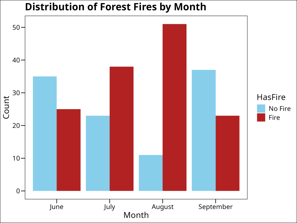
The plot shows that fires are more likely to occur in July and August. These can potentially be used as predictors in our model.
Next, let’s examine the distribution of weather variables in fire versus no-fire conditions using density plots and histograms.
# Examine the distribution of weather variables
p1 <- ggplot(df_forest_fires, aes(x = Temperature, fill = HasFire)) +
  geom_density(alpha = 0.7) +
  scale_fill_manual(values = c("No Fire" = "skyblue", "Fire" = "firebrick")) +
  labs(
    title = "Temperature Distribution",
    x = "Temperature (°C)"
  ) +
  ggthemes::theme_base()

p2 <- ggplot(df_forest_fires, aes(x = RelativeHumidity, fill = HasFire)) +
  geom_density(alpha = 0.7) +
  scale_fill_manual(values = c("No Fire" = "skyblue", "Fire" = "firebrick")) +
  labs(
    title = "Relative Humidity Distribution",
    x = "Relative Humidity (%)"
  ) +
  ggthemes::theme_base()

p3 <- ggplot(df_forest_fires, aes(x = WindSpeed, fill = HasFire)) +
  geom_density(alpha = 0.7) +
  scale_fill_manual(values = c("No Fire" = "skyblue", "Fire" = "firebrick")) +
  labs(
    title = "Wind Speed Distribution",
    x = "Wind Speed (km/h)"
  ) +
  ggthemes::theme_base()

p4 <- ggplot(df_forest_fires, aes(x = Rainfall, fill = HasFire)) +
  geom_histogram(binwidth = 0.5, position = "dodge", alpha = 0.7) +
  scale_fill_manual(values = c("No Fire" = "skyblue", "Fire" = "firebrick")) +
  labs(
    title = "Rainfall Distribution",
    x = "Rainfall (mm)"
  ) +
  ggthemes::theme_base()

# Arrange the plots in a grid
gridExtra::grid.arrange(p1, p2, p3, p4, ncol = 2)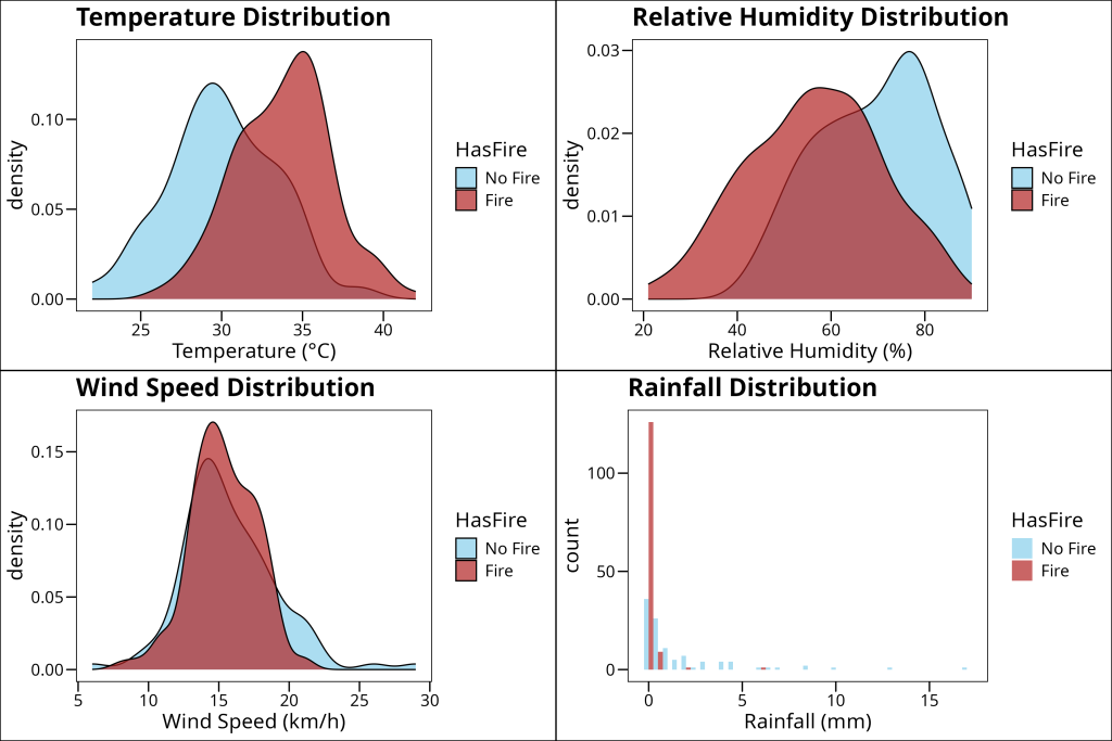
Simple Logistic Regression
Let’s start with a simple model using wind speed as a predictor:
model_ws <- glm(HasFire ~ WindSpeed,
  data = df_forest_fires,
  family = binomial(link = "logit")
)
summary(model_ws)
Call:
glm(formula = HasFire ~ WindSpeed, family = binomial(link = "logit"),
data = df_forest_fires)
Coefficients:
Estimate Std. Error z value Pr(>|z|)
(Intercept) 1.03997 0.73404 1.417 0.157
WindSpeed -0.05049 0.04650 -1.086 0.278
(Dispersion parameter for binomial family taken to be 1)
Null deviance: 332.90 on 242 degrees of freedom
Residual deviance: 331.71 on 241 degrees of freedom
AIC: 335.71
Number of Fisher Scoring iterations: 4Let’s examine the key components of the model summary:
- Coefficients:
– The intercept (1.03997) represents the log-odds of a fire when wind speed is zero
– The WindSpeed coefficient (-0.05049) indicates that for each unit increase in wind speed, the log-odds of a fire decrease by 0.05049
– The p-values (Pr(>|z|)) suggest neither coefficient is statistically significant at the α=0.05 level - Null vs. Residual Deviance:
– Null deviance (332.90) represents model fit with just an intercept
– Residual deviance (331.71) represents fit after adding WindSpeed
– The small difference suggests WindSpeed adds little predictive power - AIC (335.71):
– Used for model comparison, lower values indicate better models
– By itself, this number isn’t meaningful, but we’ll use it to compare with more complex models
Remember, since the coefficients are log odds, we can convert them to just odds by exponentiating:
\text{odds} = e^{\beta_0 + \beta_1x}In R:
exp(cbind(OddsRatio = coef(model_ws), confint(model_ws))) OddsRatio 2.5 % 97.5 %
(Intercept) 2.8291328 0.6791640 12.28138
WindSpeed 0.9507633 0.8664001 1.04093We can see that the odds of a fire occurring are 0.95. In other words, for every unit increase in wind speed, the odds of a fire remain relatively constant (95% of the previous odds).
To assess model performance, we’ll look at several metrics:
# Calculate McFadden's pseudo R-squared
null_model <- glm(HasFire ~ 1, data = df_forest_fires, family = binomial(link = "logit"))
mcfadden_r2_ws <- 1 - (logLik(model_ws) / logLik(null_model))
cat("McFadden's Pseudo R-squared for Model 1:", mcfadden_r2_ws, "\n")
McFadden's Pseudo R-squared for Model 1: 0.003577279 # Calculate accuracy
predicted_probs <- predict(model_ws, newdata = df_forest_fires, type = "response")
predicted_classes <- factor(ifelse(predicted_probs > 0.5, "Fire", "No Fire"),
levels = levels(df_forest_fires$HasFire)
)
accuracy <- sum(predicted_classes == df_forest_fires$HasFire) / nrow(df_forest_fires)
cat("Accuracy of Model 1:", accuracy, "\n")Accuracy of Model 1: 0.5967078But remember to take note of our reference!
percentage_fires <- sum(df_forest_fires$HasFire == "Fire") / nrow(df_forest_fires)
cat("Percentage of fires:", percentage_fires, "\n")
Percentage of fires: 0.563786Therefore, the accuracy is not any better than sticking to the percentage of fires itself.
Understanding the Performance Metrics:
- McFadden’s Pseudo R²:
– Values range from 0 to 1
– Our value of 0.0036 indicates the model explains very little of the variation
– Values above 0.2 are considered good fits - Classification Accuracy:
– Our model achieves 59.7% accuracy
– However, this must be compared to the baseline rate of fires (56.4%)
– The model is only performing slightly better than simply guessing “Fire” for every observation
– This illustrates why accuracy alone can be misleading – we need to consider the baseline rate in the data
Visualizing the Logistic Curve
Although this model is not very good, let us proceed nonetheless to understand how wind speed relates to fire probability by visualizing the logistic curve:
ws_range <- seq(min(df_forest_fires$WindSpeed), max(df_forest_fires$WindSpeed), length.out = 100)
predicted_probs <- predict(model_ws, newdata = data.frame(WindSpeed = ws_range), type = "response")
prob_data <- data.frame(WindSpeed = ws_range, probability = predicted_probs)

# Convert Classes back to 0/1 for plotting the raw data points
df_forest_fires$class_numeric <- as.numeric(df_forest_fires$HasFire) - 1

ggplot(prob_data, aes(x = WindSpeed, y = probability)) +
  geom_line(color = "blue", linewidth = 1.5) +
  geom_point(
    data = df_forest_fires,
    aes(x = WindSpeed, y = class_numeric, color = HasFire),
    alpha = 0.7
  ) +
  scale_color_manual(values = c("No Fire" = "skyblue", "Fire" = "firebrick")) +
  labs(
    title = "Logistic Regression Curve for Wind Speed",
    x = "Wind Speed (km/h)",
    y = "Probability of Fire"
  ) +
  ggthemes::theme_base()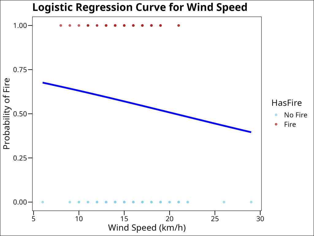
The lack of a distinct sigmoidal curve (more linear than sigmoidal) and the substantial overlap in wind speeds between fire and no-fire conditions indicate that wind speed alone is not a good predictor of fire occurrence.
Building a Better Model
Let’s improve our model by incorporating temperature, relative humidity, rainfall, and a binary indicator for August (which we expect to be the peak fire season):
model_2 <- glm(HasFire ~ IsAugust + Rainfall + RelativeHumidity + Temperature,
  data = df_forest_fires,
  family = binomial(link = "logit")
)
summary(model_2)
Call:
glm(formula = HasFire ~ IsAugust + Rainfall + RelativeHumidity +
Temperature, family = binomial(link = "logit"), data = df_forest_fires)
Coefficients:
Estimate Std. Error z value Pr(>|z|)
(Intercept) -5.31640 3.06916 -1.732 0.083238 .
IsAugust 0.08222 0.51268 0.160 0.872594
Rainfall -2.44367 0.55338 -4.416 1.01e-05 ***
RelativeHumidity -0.04137 0.01605 -2.577 0.009957 **
Temperature 0.27879 0.07994 3.487 0.000488 ***
---
Signif. codes: 0 ‘***’ 0.001 ‘**’ 0.01 ‘*’ 0.05 ‘.’ 0.1 ‘ ’ 1
(Dispersion parameter for binomial family taken to be 1)
Null deviance: 332.9 on 242 degrees of freedom
Residual deviance: 196.5 on 238 degrees of freedom
AIC: 206.5
Number of Fisher Scoring iterations: 7The improved model shows several key features:
- Temperature Effect:
– Positive coefficient indicates higher temperatures increase fire probability
– For each 1°C increase in temperature, the log odds of fire increase
– This relationship makes ecological sense as higher temperatures tend to create conditions conducive to fires - Relative Humidity Effect:
– Negative coefficient shows higher humidity reduces fire probability
– Each 1% increase in humidity decreases the log odds of fire
– This aligns with our understanding that moist conditions inhibit fire spread - Rainfall Effect:
– Strong negative relationship with fire probability
– Even small amounts of rainfall significantly reduce fire odds
– This direct measure of precipitation complements the humidity effect - August Effect:
– Positive coefficient for IsAugust indicates higher fire probability in August
– This captures the seasonal peak in fire risk
– The binary indicator helps account for unmeasured seasonal factors
Model Comparison
Let’s compare our models using several metrics:
# McFadden's pseudo R-squared
mcfadden_r2_model_2 <- 1 - (logLik(model_2) / logLik(null_model))
cat("McFadden's Pseudo R-squared for Model 2:", mcfadden_r2_model_2, "\n")
McFadden's Pseudo R-squared for Model 2: 0.4097258# Accuracy
predicted_probs <- predict(model_ws, newdata = df_forest_fires, type = "response")
predicted_classes <- factor(ifelse(predicted_probs > 0.5, "Fire", "No Fire"),
levels = levels(df_forest_fires$HasFire)
)
accuracy <- sum(predicted_classes == df_forest_fires$HasFire) / nrow(df_forest_fires)
cat("Accuracy of Model 2:", accuracy, "\n")Accuracy of Model 2: 0.8477366Before comparing our models using deviance and AIC, let’s understand what these metrics tell us about model performance:
- Deviance is a measure of model fit that generalizes the concept of sum of squared residuals to GLMs:
- Null deviance shows how well the response variable is predicted by a model with just an intercept (the null model)
- Residual deviance shows how well the response is predicted by the model when including the predictors
- The difference between null and residual deviance follows a chi-square distribution, allowing us to test whether adding predictors significantly improves the model
- AIC (Akaike Information Criterion) helps us compare models by balancing model fit against complexity:
- AIC = -2(log-likelihood) + 2(number of parameters)
- The first term decreases with better fit, while the second term increases with model complexity
- Lower AIC values indicate better models
- A difference of 2 AIC units is considered meaningful, with the lower AIC model being preferred
Both metrics are particularly useful for GLMs because, unlike R² in linear regression, they are based on the model’s likelihood and thus account for the non-normal error distribution in logistic regression.
# Compare deviance
anova(model_ws, model_2, test = "Chisq")
Analysis of Deviance Table
Model 1: HasFire ~ WindSpeed
Model 2: HasFire ~ IsAugust + Rainfall + RelativeHumidity + Temperature
Resid. Df Resid. Dev Df Deviance Pr(>Chi)
1 241 331.71
2 238 196.50 3 135.21 < 2.2e-16 ***
---
Signif. codes: 0 ‘***’ 0.001 ‘**’ 0.01 ‘*’ 0.05 ‘.’ 0.1 ‘ ’ 1The deviance comparison shows that Model 2 significantly reduces the residual deviance by 135.21 units (p < 2.2e-16). This substantial reduction in deviance indicates that adding temperature, relative humidity, rainfall, and the August indicator significantly improves the model’s fit compared to using wind speed alone.
# Compare AIC
AIC(model_ws, model_2)
df AIC
model_ws 2 335.7131
model_2 5 206.5046The AIC comparison reinforces this conclusion. Model 2’s AIC (206.5) is substantially lower than Model 1’s AIC (335.7). The difference of 129.2 AIC units strongly suggests that Model 2 provides a much better balance of model fit and complexity. Generally, a difference of more than 2 AIC units is considered meaningful, and here we have a difference of over 100 units.
Looking at the odds ratios, we can interpret the effects of each predictor:
- Temperature: For each 1°C increase in temperature, the odds of fire increase by 32% (OR = 1.32, 95% CI: 1.14-1.56)
- Relative Humidity: Each 1% increase in humidity reduces the odds of fire by about 4% (OR = 0.96, 95% CI: 0.93-0.99)
- Rainfall: The odds ratio of 0.087 indicates that each mm of rainfall reduces the odds of fire by about 91% (1 – 0.087 = 0.913). This strong negative effect makes ecological sense as wet conditions significantly inhibit fire occurrence
- August: Being in August increases the odds of fire by about 9% (OR = 1.09), though this effect is not statistically significant (95% CI: 0.40-3.07)
When interpreting these coefficients, it’s important to note that R treats different variable types distinctly:
- Continuous variables (Temperature, RelativeHumidity, Rainfall): The coefficients represent the change in log odds for a one-unit increase in the predictor
- Binary indicators (IsAugust): The coefficient represents the change in log odds when the indicator changes from 0 to 1
- Nominal Factors: R uses dummy/treatment coding by default, where one level serves as the reference category. The coefficients represent the change in log odds relative to this reference level
- Ordinal Factors: R uses polynomial coding by default, with suffixes like
.Lfor linear,.Qfor quadratic, and.Cfor cubic terms. The coefficients represent linear, quadratic, and cubic changes to the log odds per unit change in the predictor, respectively.
Visualizing the effects of multiple predictors in logistic regression can be challenging because the relationship between each predictor and the response depends on the values of other predictors. The plots below, generated using the ggeffects package, show the marginal effects of each predictor while holding other variables at their mean or reference values:
ggeffects::ggeffect(model_2) %>%
  plot() %>%
  sjPlot::plot_grid(tags = FALSE) +
  ggthemes::theme_base()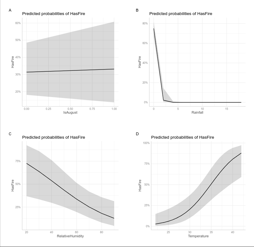
Making Predictions
To demonstrate the practical application of our model, let’s examine some scenarios. We’ve created scenarios that vary in rainfall amount and month (August vs. July) while holding temperature and relative humidity constant at moderate levels. This allows us to see how these key factors influence fire probability:
scenarios <- data.frame(
  Scenario = c(
    "No rain in August",
    "Light drizzle in August",
    "Heavy rain in August",
    "No rain in July",
    "Light drizzle in July",
    "Heavy rain in July"
  ),
  Rainfall = c(0, 1, 10, 0, 1, 10),
  Temperature = c(20, 20, 20, 20, 20, 20),
  IsAugust = c(1, 1, 1, 0, 0, 0),
  RelativeHumidity = c(50, 50, 50, 50, 50, 50)
)

# Add month as a descriptive column and for color coding when plotting
scenarios$Month <- c("August", "August", "August", "July", "July", "July")

# Predict probabilities
scenarios$Fire_Probability <- predict(model_2, newdata = scenarios, type = "response")

# Display the scenarios and their predicted probabilities
scenarios %>%
  select(Scenario, Month, Rain, Fire_Probability) %>%
  mutate(Fire_Probability = scales::percent(Fire_Probability, accuracy = 0.1))
Scenario Month Rainfall Temperature RelativeHumidity Fire_Probability
1 No rain in August August 0 20 50 15.1%
2 Light drizzle in August August 1 20 50 1.5%
3 Heavy rain in August August 10 20 50 0.0%
4 No rain in July July 0 20 50 14.1%
5 Light drizzle in July July 1 20 50 1.4%
6 Heavy rain in July July 10 20 50 0.0%Or, as a figure:
ggplot(
  scenarios,
  aes(x = reorder(Scenario, -Fire_Probability), y = Fire_Probability, fill = Month)
) +
  geom_col() +
  geom_text(aes(label = scales::percent(Fire_Probability, accuracy = 0.1)), vjust = -0.5) +
  scale_fill_manual(values = c("August" = "orange", "July" = "skyblue")) +
  labs(
    title = "Predicted Fire Probability for Different Scenarios",
    x = NULL,
    y = "Probability of Fire"
  ) +
  ggthemes::theme_base() +
  theme(axis.text.x = element_text(angle = 45, hjust = 1))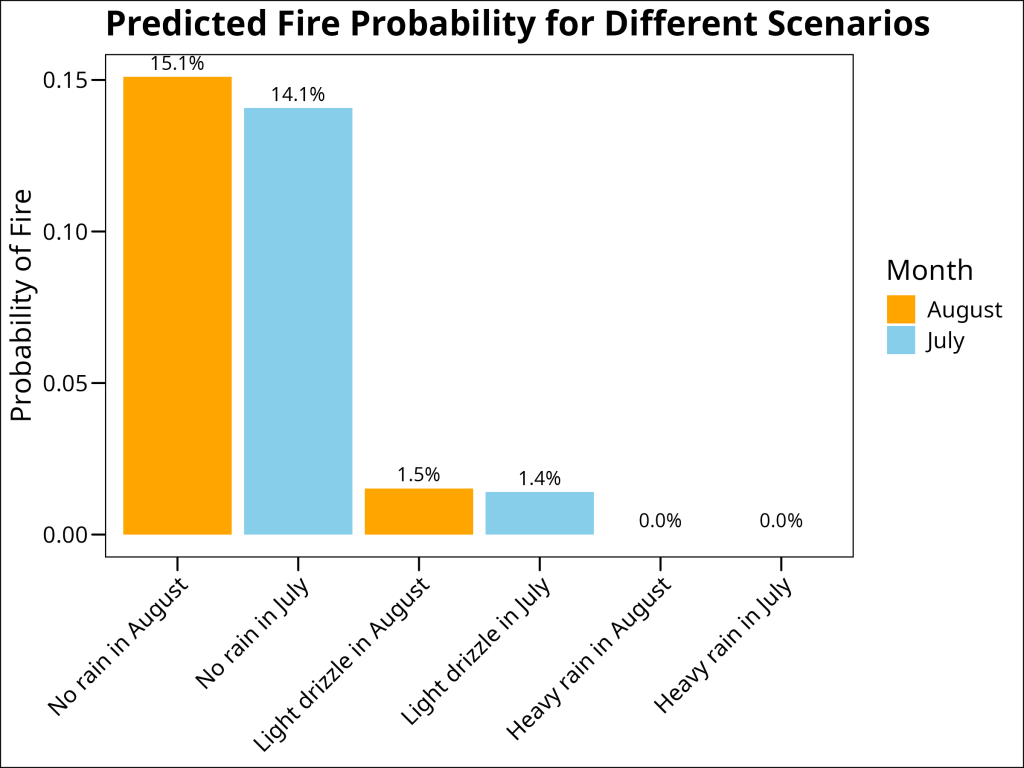
Practical Applications and Limitations
While our model provides insights into fire occurrence, it’s important to recognize its limitations:
- Assumptions:
- Independence of observations
- Linear relationship between predictors and log odds
- No perfect multicollinearity among predictors
- Practical Limitations:
- Weather variables may interact in complex ways not captured by the model
- Temporal autocorrelation may violate independence assumption
- Other important predictors (e.g., vegetation condition) are not included
- Prediction Challenges:
- Model accuracy varies across different conditions
- Extreme weather events may be underrepresented
- Spatial variation in fire susceptibility is not considered
Conclusion
Logistic regression provides a powerful framework for analyzing binary outcomes in ecological data. Through our forest fire example, we’ve seen how to:
- Build and interpret logistic regression models
- Transform between probabilities, odds, and log odds
- Evaluate model performance using multiple metrics
- Consider practical limitations and assumptions
This statistical tool is valuable for many ecological applications, from species distribution modeling to behavioral studies. Understanding both its power and limitations helps ensure appropriate application in research contexts.