Untangling Statistical Power: The Basics

Before diving deep, let’s refresh a core idea from hypothesis testing. We typically start with a null hypothesis (H₀), which is a statement of no effect or no difference (e.g., “predator cues have no effect on guppy fin length”). We then propose an alternative hypothesis (H₁), which states that there is an effect (e.g., “predator cues do affect guppy fin length”). Our statistical tests then help us decide which hypothesis is better supported by our data.

Now, how does power analysis fit into this? Think of it as a delicate balancing act involving four key ingredients that determine the success of our “expedition”: the size of the creature we’re looking for (effect size), the number of explorers we send out (sample size), our willingness to mistakenly claim we saw a creature when it wasn’t there (Type I error or alpha), and our ability to actually spot the creature if it’s present (statistical power).

The Key Ingredients of Power

Let’s consider these ingredients more closely. First, we have effect size. This quantifies the magnitude of the phenomenon we’re investigating. Is the change in fin length due to predator cues a tiny, almost imperceptible flicker, or a dramatic, easily noticeable transformation? A very small effect is like trying to hear a whisper in a crowded room – you’ll need to listen very carefully (i.e., have a very sensitive study) to detect it. A large effect is more like a shout – much easier to pick up. Effect size is independent of sample size and tells us about the practical or biological significance of our findings.

Next is our significance level, commonly known as alpha (\(\alpha\)). This is a threshold we set, typically at 0.05 (or 5%). It represents our tolerance for making a Type I error. A Type I error occurs if we reject the null hypothesis when it’s actually true – essentially, a “false positive.” It’s like claiming you found your elusive creature when, in reality, it was just a rustling in the bushes. Setting \(\alpha\) at 0.05 means we accept a 5% chance of making such a mistake.

Then there’s the flip side: a Type II error, denoted by beta (\(\beta\)). This happens when we fail to reject the null hypothesis when it’s actually false – a “false negative.” In our analogy, this means the creature was indeed there, but our expedition missed it. Perhaps our tools weren’t sensitive enough, or we didn’t look in the right places for long enough.

This brings us to the star of the show: statistical power. Power is defined as 1 – \(\beta\). It’s the probability that our study will correctly detect an effect that is truly present. If our study has 80% power, it means that if a real effect of a certain size exists, we have an 80% chance of our statistical test yielding a significant result and correctly rejecting the null hypothesis. We want our studies to have high power, typically 80% or greater, to ensure we have a good chance of finding what we’re looking for, if it’s there.

Finally, sample size (N) – the number of observations or participants in our study – plays a huge role. Generally, the larger our sample size, the more information we have, and the easier it becomes to detect an effect, thus increasing our power. It’s like sending out more explorers or giving them more time; it increases the chances of making a discovery.

Visualizing the Concepts

The interplay between these concepts can be visualized with two overlapping distributions, as shown in the image below. Imagine one distribution represents the world if the null hypothesis is true (no effect), and the other represents the world if the alternative hypothesis is true (an effect of a specific size exists).

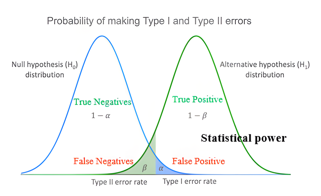
The null hypothesis distribution (often depicted on the left) shows the range of sample outcomes we’d expect if there’s truly no effect. The alternative hypothesis distribution (often to the right, indicating an effect) shows outcomes if there is a real effect of a certain magnitude. The distance between the peaks of these two distributions is related to the effect size – larger effects mean more separation.

Our significance level, \(\alpha\), is a cutoff point we define on the null distribution. If our study’s result falls into the \(\alpha\) region (the blue area in the image, typically in the tail), we reject the null hypothesis. This area represents the probability of a Type I error (a false positive). The remaining area under the null distribution (1 – \(\alpha\)) represents true negatives – correctly concluding there’s no effect when none exists.

Now, look at the alternative distribution. The portion of this distribution that falls on the “wrong” side of our \(\alpha\) cutoff (i.e., where we would not reject the null hypothesis, even though the alternative is true) is \(\beta\) (the green area). This is our chance of a Type II error (a false negative). The rest of the area under the alternative distribution represents our statistical power (1 – \(\beta\)). This is the probability of correctly detecting a true effect – a true positive!

Power analysis, typically done before conducting a study, helps us manipulate these elements, most commonly by adjusting the sample size, to achieve a desired level of power given an expected effect size and our chosen alpha level. It helps answer questions like, “How many guppies do I need to study to have an 80% chance of detecting a meaningful change in fin length?” This proactive planning is essential for efficient and informative research.

It is crucial to understand that performing power analysis after data has been collected (often called post-hoc power analysis) to interpret non-significant results is generally not informative and is STRONGLY discouraged.

Planning Our Guppy Study: A Practical Example

Now that we’ve covered the conceptual groundwork of power analysis, let’s apply it to a practical scenario. Imagine we are researchers – perhaps a professor and their students – keen on understanding how guppies (Poecilia reticulata) adapt their physical features in response to predators. Specifically, we’re interested in predator-induced plasticity in their caudal (tail) fin morphology. We also hypothesize that the complexity of their environment, such as the amount of refuge available, might influence this plastic response. Before we can even begin our experiment, a critical question arises: how many guppies do we actually need to order from our animal supplier to run a meaningful study? This is where power analysis becomes indispensable. We don’t want to order too few and miss a real effect, nor do we want to order too many, which would be wasteful and ethically questionable.

The core question for our power analysis will be: “Given our research design and the statistical tests we plan to use (like t-tests to compare predator vs. control, or ANOVA to look at refuge effects, and more complex linear models for interactions), what sample size per group will give us a good chance (e.g., 80% power) of detecting an effect if it’s truly there, assuming a certain effect size?” Let’s dive into how we can use R to answer this.

Power Analysis in R with the pwr Package

To perform power analysis in R, one of the most straightforward and commonly used packages is pwr. If you haven’t used it before, you’ll need to install it first by running install.packages("pwr") in your R console. Once installed, we can load it into our R session.

library(pwr)

Throughout our guppy study example, we’ll work with some standard conventions for our desired statistical properties. We’ll set our significance level (alpha) to 0.05, which is a common choice in many scientific fields. We’ll also aim for a statistical power of 80%. This means we want an 80% chance of detecting an effect if it truly exists. Remember, power is 1 – \(\beta\), so an 80% power corresponds to a \(\beta\) of 0.20 (a 20% chance of a Type II error).

alpha <- 0.05 # Significance level (Type I error rate)
beta <- 0.20  # Type II error rate (1 - desired power)
desired_power <- 1 - beta # Desired statistical power

Power Analysis for T-Tests

Let’s start with a common scenario: comparing the means of two groups using a t-test. In our guppy study, a primary question might be: “Is there a significant difference in mean caudal fin length between guppies exposed to predator cues and those in a control group?”

For t-tests, the effect size is typically expressed as Cohen’s d. Cohen’s d measures the difference between two means in terms of standard deviations. Think of it as a standardized way to say how far apart the two group means are. General (and somewhat arbitrary) guidelines for interpreting Cohen’s d are:

• d = 0.2: Small effect
• d = 0.5: Medium effect
• d = 0.8: Large effect

Deciding on an expected effect size is often the trickiest part of power analysis. It might come from previous research, a pilot study, or the smallest effect size that you would consider biologically meaningful.

Calculating Sample Size (n per group)

Let’s say, based on some preliminary work or literature, we expect a medium effect size (d = 0.5) for the difference in fin length due to predator exposure. How many guppies would we need per group (predator-exposed and control) to achieve our desired 80% power at an alpha of 0.05?

# For medium effect (d=0.5)
power_t_test_n_medium_results <- pwr.t.test(
  d = 0.5,
  sig.level = alpha,
  power = desired_power,
  type = "two.sample",        # We are comparing two independent groups
  alternative = "two.sided" # We are interested if means are different (could be larger or smaller)
)
power_t_test_n_medium_results

     Two-sample t test power calculation 

              n = 63.76561
              d = 0.5
      sig.level = 0.05
          power = 0.8
    alternative = two.sided

NOTE: n is number in *each* group

The output tells us that n = 63.76561. Since we can’t have fractions of guppies, we would round this up. So, we’d need approximately 64 guppies per group (for a total of 128 guppies) to detect a medium effect size with 80% power.

Now, what if we suspect the effect might be smaller? Let’s see what happens if we aim to detect a small effect size (d = 0.2) with the same power and alpha:

# For small effect (d=0.2)
power_t_test_n_small_results <- pwr.t.test(
  d = 0.2,
  sig.level = alpha,
  power = desired_power,
  type = "two.sample",
  alternative = "two.sided"
)
power_t_test_n_small_results

     Two-sample t test power calculation 

              n = 393.4057
              d = 0.2
      sig.level = 0.05
          power = 0.8
    alternative = two.sided

NOTE: n is number in *each* group

Wow, that’s a big jump! To detect a small effect size, we would need approximately 394 guppies per group (a total of 788 guppies). This illustrates a fundamental principle: detecting smaller effects requires substantially larger sample sizes to achieve the same statistical power. This is because a smaller effect is harder to distinguish from random sampling variation, so you need more data to be confident it’s real.

Calculating Power Given a Fixed Sample Size

Sometimes, practical constraints limit our sample size. Perhaps we only have funding or tank space for, say, 50 guppies per group. If we stick with our expectation of a medium effect size (d = 0.5), what would our statistical power be with this limited sample size?

n_t_test_example <- 50 # Example n per group

power_t_test_check_results <- pwr.t.test(
  d = 0.5,
  n = n_t_test_example,
  sig.level = alpha,
  type = "two.sample",
  alternative = "two.sided"
)
power_t_test_check_results

     Two-sample t test power calculation 

              n = 50
              d = 0.5
      sig.level = 0.05
          power = 0.6968934
    alternative = two.sided

NOTE: n is number in *each* group

With 50 guppies per group, our power to detect a medium effect size drops to approximately 0.697, or about 70%. This is below our desired 80% power, meaning we’d have a higher chance (around 30%) of missing a true medium effect if it exists (a Type II error).

Calculating Minimum Detectable Effect Size

Let’s flip the question again. If we are constrained to 50 guppies per group and we insist on achieving our desired 80% power, what is the smallest effect size (minimum Cohen’s d) we could reliably detect?

effect_t_test_check_results <- pwr.t.test(
  n = n_t_test_example, # Still 50 per group
  sig.level = alpha,
  power = desired_power, # Our target 80% power
  type = "two.sample",
  alternative = "two.sided"
)
effect_t_test_check_results

     Two-sample t test power calculation 

              n = 50
              d = 0.565858
      sig.level = 0.05
          power = 0.8
    alternative = two.sided

NOTE: n is number in *each* group

This tells us that with 50 guppies per group and aiming for 80% power, the smallest effect we could hope to consistently detect is a Cohen’s d of approximately 0.57. If the true effect size is smaller than this, say d = 0.5 (our original medium effect), we wouldn’t have 80% power to detect it with this sample size. This kind of calculation is very useful for understanding the limitations of a study given fixed resources.

Power Analysis for One-Way ANOVA

Our guppy study also involves comparing mean fin lengths across more than two groups. For instance, we have three levels of refuge availability (low, medium, high). A one-way Analysis of Variance (ANOVA) is the appropriate test for this. The pwr package can help us plan for this too.

For ANOVA, a common effect size measure is Cohen’s f. Conceptually, Cohen’s f relates to the standard deviation of the group means divided by the common within-group standard deviation. It quantifies how much the group means differ relative to the variation within the groups. Similar to Cohen’s d, there are conventional (and again, somewhat arbitrary) benchmarks for Cohen’s f:

• f = 0.10: Small effect
• f = 0.25: Medium effect
• f = 0.40: Large effect

Let’s assume we’re interested in the effect of the three refuge levels on guppy fin length.

k_anova_groups <- 3 # Number of groups (e.g., 3 refuge levels)

Calculating Sample Size (n per group)

Suppose we anticipate a medium effect size (f = 0.25) for the differences in fin length among the three refuge conditions. How many guppies would we need per refuge condition to achieve our 80% power target?

power_anova_n_medium_results <- pwr.anova.test(
  k = k_anova_groups,
  f = 0.25, # Medium effect size
  sig.level = alpha,
  power = desired_power
)
power_anova_n_medium_results

     Balanced one-way analysis of variance power calculation 

              k = 3
              n = 52.3966
              f = 0.25
      sig.level = 0.05
          power = 0.8

NOTE: n is number in each group

The output indicates n = 52.3966. Rounding up, we’d need approximately 53 guppies per refuge group. Since we have 3 refuge groups, this would mean a total of \(53 \times 3 = 159\) guppies for this part of the study, assuming this was the only factor.

Calculating Power Given a Fixed Sample Size

What if our resources limit us to, say, 40 guppies per refuge condition? If we still expect a medium effect size (f = 0.25), what would our statistical power be?

n_anova_example_per_group <- 40 # Example n per group

power_anova_check_results <- pwr.anova.test(
  k = k_anova_groups,
  n = n_anova_example_per_group,
  f = 0.25, # Medium effect size
  sig.level = alpha
)
power_anova_check_results

     Balanced one-way analysis of variance power calculation 

              k = 3
              n = 40
              f = 0.25
      sig.level = 0.05
          power = 0.6756745

NOTE: n is number in each group

With 40 guppies in each of the 3 refuge groups, our power to detect a medium effect size is about 0.676, or roughly 68%. Again, this is less than our desired 80%, indicating a considerable risk of failing to detect a true medium-sized difference between the refuge groups.

Calculating Minimum Detectable Effect Size

Finally, if we are fixed at 40 guppies per group and want to maintain 80% power, what’s the smallest effect size (minimum Cohen’s f) we could reliably detect among the three refuge levels?

effect_anova_check_results <- pwr.anova.test(
  k = k_anova_groups,
  n = n_anova_example_per_group, # Still 40 per group
  sig.level = alpha,
  power = desired_power       # Our target 80% power
)
effect_anova_check_results

     Balanced one-way analysis of variance power calculation 

              k = 3
              n = 40
              f = 0.2870219
      sig.level = 0.05
          power = 0.8

NOTE: n is number in each group

This result shows that with 40 guppies per group, we would have 80% power to detect an effect size (Cohen’s f) of about 0.287 or larger. If the true differences between the refuge groups correspond to an effect size smaller than this (e.g., our anticipated medium effect of f = 0.25), our power would be less than 80%.

This kind of calculation is vital. It tells us the limits of our detection ability for a given experimental setup. If we anticipate an effect smaller than f=0.29 but can only manage 40 fish per group, we might need to reconsider our design or acknowledge the lower power for smaller effects.

Power Analysis for General Linear Models (GLM) / Multiple Regression

Often, our research questions are more complex and involve multiple predictor variables, or covariates, influencing an outcome. This is where General Linear Models (GLMs), including multiple regression, come into play. For our guppy study, we might want to model fin length as a function of predator exposure, refuge availability, and the guppy’s initial body size simultaneously.

The pwr package provides the pwr.f2.test() function for power analysis in the context of GLMs. The effect size used here is Cohen’s f². Cohen’s f² quantifies the proportion of variance explained by a set of predictors relative to the unexplained variance. It’s calculated as:

f² = R² / (1 – R²)

Where R² is the coefficient of determination for the predictors of interest. Guidelines for f² are:

• f² = 0.02: Small effect
• f² = 0.15: Medium effect
• f² = 0.35: Large effect

The key parameters for pwr.f2.test() are:

• u: Numerator degrees of freedom. This is the number of predictors whose combined effect you are testing.
• v: Denominator degrees of freedom. This is calculated as N – p_full – 1, where N is the total sample size and p_full is the total number of predictors in the full model (excluding the intercept). When solving for sample size, the function directly gives you v, and you then calculate N.
• f2: The anticipated effect size (Cohen’s f²).
• sig.level: Significance level (alpha).
• power: Desired statistical power.

Scenario 1: Power for an Overall Model’s R-squared

Let’s consider a model where we want to predict guppy fin length using predator exposure (a binary predictor), refuge availability (which, with 3 levels, would typically be represented by 2 dummy variables in a GLM), and initial body size (a continuous covariate). So, we have 1 (predator) + 2 (refuge) + 1 (body size) = 4 predictors in total whose combined contribution we’re interested in.

Our question: How many guppies (total sample size N) do we need to detect a medium effect (f² = 0.15) for this set of 4 predictors, with 80% power and an alpha of 0.05?

Here, u (numerator degrees of freedom) = 4 (for the 4 predictors we are evaluating together).

# Effect sizes for Cohen's f2 (regression)
cohen_f2_medium_glm <- 0.15

# Scenario 1: Power for an overall model's R-squared
# Model: fin_length ~ predator + refuge_L + refuge_M + body_size
u_model1 <- 1 + 2 + 1 # = 4 predictors (numerator df for the set of predictors)

# Calculate v (denominator df) for medium effect (f2=0.15)
calc_v_model1_medium_results <- pwr.f2.test(
  u = u_model1,
  f2 = cohen_f2_medium_glm,
  sig.level = alpha,
  power = desired_power
)
calc_v_model1_medium_results

 Multiple regression power calculation 

          u = 4
          v = 79.44992
         f2 = 0.15
  sig.level = 0.05
      power = 0.8

The function gives us v = 79.44992. To find the total sample size N, we use the formula v = N – u – 1. Rearranging this gives N = v + u + 1.

N_model1_medium <- ceiling(calc_v_model1_medium_results$v) + u_model1 + 1
N_model1_medium

[1] 85

So, we would need a total sample size of approximately 85 guppies to achieve 80% power to detect a medium effect (f² = 0.15) for this specific GLM involving predator cues, refuge availability, and body size.

Scenario 2: Power for a Specific Interaction Term

Sometimes, we are particularly interested in the effect of specific terms within a larger model, such as an interaction. For instance, in our guppy study, we might hypothesize that the effect of predator cues on fin length depends on the level of refuge availability. This would be tested with a `Predator * Refuge` interaction term.

Let’s consider a full model: `fin_length ~ Predator + Refuge + BodySize + Predator*Refuge`.

The `Predator` term has 1 df (2 levels – 1). The `Refuge` term has 2 df (3 levels – 1). The `Predator*Refuge` interaction term’s degrees of freedom is the product of the df of the main effects involved: (2-1) * (3-1) = 1 * 2 = 2. So, for testing the interaction, u = 2.

How many guppies (total sample size N) would we need to detect a medium effect (f² = 0.15) specifically for this interaction term, with 80% power and an alpha of 0.05?

# Scenario 2: Power for a specific interaction term
# Full model considered: fin_length ~ Predator + Refuge + BodySize + Predator*Refuge
# p_full_scenario2 <- 1 + 2 + 1 + 2 # df for P, R, BS, P*R (total predictors in model, excluding intercept, if we consider body size fixed)
# Actually, the pwr.f2.test focuses on the 'u' predictors against the error variance from the rest.
# The total number of predictors in the model (p_full) is needed to calculate N from v.
# Predictor DFs: P(1), R(2), BS(1), P*R interaction(2). So p_full = 1+2+1+2 = 6 for this model.

u_PR_interaction <- 2 # df for the Predator*Refuge interaction term

calc_v_PR_medium_results <- pwr.f2.test(
  u = u_PR_interaction,
  f2 = cohen_f2_medium_glm, # using the same medium effect size
  sig.level = alpha,
  power = desired_power
)
calc_v_PR_medium_results

 Multiple regression power calculation 

          u = 2
          v = 66.63869
         f2 = 0.15
  sig.level = 0.05
      power = 0.8

The function returns v = 66.63869. Now, to calculate N, we need u (which is 2 for the interaction term) and p_full, the total number of predictors in the model that includes the interaction. The model is `fin_length ~ Predator + Refuge + BodySize + Predator*Refuge`. The predictors are:

• Predator (1 df)
• Refuge (2 df, from 3 levels)
• BodySize (1 df)
• Predator*Refuge interaction (2 df)

So, the total number of predictor degrees of freedom in this model, p_full, is 1 + 2 + 1 + 2 = 6.

The formula for v in pwr.f2.test is v = N – u – p_others – 1, where p_others are the predictors *not* included in u. More simply, v = N – p_{full_model_df} – 1, where p_{full_model_df} are the degrees of freedom for all terms in the model (equivalent to p_full as defined above). So, N = v + p_{full_model_df} + 1.

# p_full for the model: fin_length ~ Predator + Refuge + BodySize + Predator*Refuge
# Predator (1 df) + Refuge (2 df) + BodySize (1 df) + P*R (2 df) = 6 df
p_full_scenario2 <- 1 + 2 + 1 + 2

N_PR_interaction_medium <- ceiling(calc_v_PR_medium_results$v) + p_full_scenario2 + 1
N_PR_interaction_medium

[1] 74

To detect a medium effect (f² = 0.15) for the Predator*Refuge interaction term (which has u=2 df) with 80% power, within the context of our full model (which has a total of p_full=6 predictor df), we would need a total sample size of approximately 74 guppies.

It’s interesting to note that this is less than the N=85 calculated for the overall R-squared of the simpler model in Scenario 1. This happens because here u (the df for the effect of interest) is smaller (2 vs 4). Generally, for a given effect size (f2), testing an effect with fewer degrees of freedom (a more specific hypothesis) requires fewer subjects than testing an effect with more degrees of freedom (a more general hypothesis, like overall model fit).

These examples highlight how power analysis for GLMs allows us to plan for complex designs, whether we’re interested in the overall predictive power of a model or the significance of specific predictors or interactions within it. The key is to carefully define u (the number of parameters you are testing) and correctly calculate N from the resulting v based on the total number of parameters in your specific model.

Summary

• Purpose of Power Analysis: To determine the probability that a statistical test will detect an effect of a certain size if it truly exists, before the study is conducted. It helps in deciding the optimal sample size.
• Core Components: Statistical power is determined by the interplay of four factors: effect size, sample size (N), significance level (\(\alpha\)), and the desired power (1 – \(\beta\)).
• Post-hoc Power Analysis: Performing power analysis after data has been collected to interpret non-significant results is generally not informative and is STRONGLY discouraged.
• Effect Size is Crucial: Estimating or hypothesizing a biologically meaningful effect size is often the most challenging, yet most critical, input for power analysis. Smaller effects require larger sample sizes to detect.
• Sample Size Trade-offs: Increasing sample size generally increases power, but this must be balanced against practical constraints like cost, time, and ethical considerations regarding the use of subjects.
• The pwr Package in R: Provides versatile functions (pwr.t.test, pwr.anova.test, pwr.f2.test, etc.) to calculate power, sample size, or minimum detectable effect size for various common statistical tests.
• A Priori Planning: Power analysis should be performed before data collection to inform study design, not as an afterthought.
• Limitations: Power analysis relies on assumptions and estimates (especially for effect size). The calculated power is only as good as these inputs. It doesn’t guarantee that an effect will be found, only the probability of detecting it if it exists at the specified magnitude.

By thoughtfully considering these aspects and utilizing tools like the pwr package in R, researchers in ecology, evolutionary biology, and beyond can enhance the rigor and efficiency of their scientific investigations. Happy researching!