Introduction

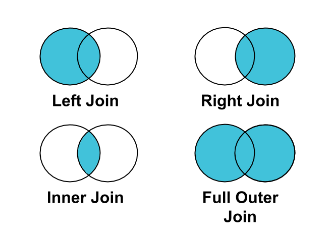
Joins are operations that combine rows from two or more tables based on related columns. These operations are fundamental when working with data spread across multiple tables. The main types of joins include:

• Inner join: Returns only the rows that have matching values in both tables
• Left join: Returns all rows from the left table and matching rows from the right table
• Right join: Returns all rows from the right table and matching rows from the left table
• Full join (outer join): Returns all rows when there is a match in either the left or right table

In ecological and evolutionary biology research, joining tables is essential in numerous contexts:

• Genomic studies: Combining gene annotation data with expression levels or conservation scores
• Phylogenetic research: Merging species trait data with evolutionary relationships
• Microbiome analysis: Connecting taxonomic information with abundance data and sample metadata
• Long-term ecological monitoring: Integrating environmental measurements with species observation data
• Biodiversity assessments: Linking specimen data with geographic and climate information

Joining Tables

Data Preparation

To demonstrate join operations, we’ll create three evolutionary biology datasets related to genes and their properties. These datasets represent a realistic scenario where researchers might study gene conservation and expression patterns across different species:

• df_genes: Contains basic information about genes, including their names, chromosomal locations, and functional categories
• df_expression: Contains gene expression levels measured in different species and tissues
• df_conservation: Contains evolutionary conservation scores and information about when genes originated

# Gene information dataset (contains gene IDs and their functions)
df_genes <- tibble(
  gene_id = c("FOXP2", "BRCA1", "CFTR", "MC1R", "OCA2", "HERC2"),
  gene_name = c(
    "Forkhead Box P2", "Breast Cancer 1", "Cystic Fibrosis Transmembrane Conductor",
    "Melanocortin 1 Receptor", "Oculocutaneous Albinism II", "HECT and RLD Domain Containing E3 Ligase 2"
  ),
  chromosome = c(7, 17, 7, 16, 15, 15),
  function_category = c(
    "Transcription factor", "Tumor suppressor", "Ion channel",
    "Receptor", "Transport protein", "E3 ubiquitin ligase"
  )
)
df_genes

# A tibble: 6 × 4
  gene_id gene_name                                  chromosome function_category   
  <chr>   <chr>                                           <dbl> <chr>               
1 FOXP2   Forkhead Box P2                                     7 Transcription factor
2 BRCA1   Breast Cancer 1                                    17 Tumor suppressor    
3 CFTR    Cystic Fibrosis Transmembrane Conductor             7 Ion channel         
4 MC1R    Melanocortin 1 Receptor                            16 Receptor            
5 OCA2    Oculocutaneous Albinism II                         15 Transport protein   
6 HERC2   HECT and RLD Domain Containing E3 Ligase 2         15 E3 ubiquitin ligase 

# Species df_expression dataset (contains gene expression levels in different species)
df_expression <- tibble(
  gene_id = c("FOXP2", "FOXP2", "FOXP2", "BRCA1", "BRCA1", "MC1R", "MC1R", "OCA2", "HERC2", "SLC24A5"),
  species = c(
    "Homo sapiens", "Pan troglodytes", "Mus musculus", "Homo sapiens", "Mus musculus",
    "Homo sapiens", "Canis lupus", "Homo sapiens", "Homo sapiens", "Homo sapiens"
  ),
  expression_level = c(15.2, 12.1, 9.8, 22.5, 18.7, 8.9, 14.3, 5.6, 11.2, 7.8),
  tissue = c("Brain", "Brain", "Brain", "Breast", "Breast", "Skin", "Skin", "Eye", "Eye", "Skin")
)
df_expression

# A tibble: 10 × 4
   gene_id species         expression_level tissue
   <chr>   <chr>                      <dbl> <chr> 
 1 FOXP2   Homo sapiens                15.2 Brain 
 2 FOXP2   Pan troglodytes             12.1 Brain 
 3 FOXP2   Mus musculus                 9.8 Brain 
 4 BRCA1   Homo sapiens                22.5 Breast
 5 BRCA1   Mus musculus                18.7 Breast
 6 MC1R    Homo sapiens                 8.9 Skin  
 7 MC1R    Canis lupus                 14.3 Skin  
 8 OCA2    Homo sapiens                 5.6 Eye   
 9 HERC2   Homo sapiens                11.2 Eye   
10 SLC24A5 Homo sapiens                 7.8 Skin  

df_conservation <- tibble(
  gene_id = c("FOXP2", "BRCA1", "CFTR", "MC1R", "OCA2", "SLC24A5", "TYR"),
  conservation_score = c(0.92, 0.88, 0.85, 0.76, 0.81, 0.74, 0.79),
  last_common_ancestor = c("Amniotes", "Mammals", "Mammals", "Vertebrates", "Vertebrates", "Vertebrates", "Vertebrates"),
  millions_years_ago = c(312, 125, 125, 500, 500, 500, 500)
)
df_conservation

# A tibble: 7 × 4
  gene_id conservation_score last_common_ancestor millions_years_ago
  <chr>                <dbl> <chr>                             <dbl>
1 FOXP2                 0.92 Amniotes                            312
2 BRCA1                 0.88 Mammals                             125
3 CFTR                  0.85 Mammals                             125
4 MC1R                  0.76 Vertebrates                         500
5 OCA2                  0.81 Vertebrates                         500
6 SLC24A5               0.74 Vertebrates                         500
7 TYR                   0.79 Vertebrates                         500

Inner Joins

An inner join returns only the rows where there is a match in both tables based on the specified key column(s). This is useful when you want to analyze only the data that has complete information in both datasets.

In evolutionary biology, inner joins are often used when you want to focus on genes or species that have complete information across multiple datasets. For example, you might use an inner join to analyze only genes that have both expression data and functional annotations.

df_genes_expr_inner <- inner_join(df_genes, df_expression, by = "gene_id")
df_genes_expr_inner

# A tibble: 9 × 7
  gene_id gene_name                                  chromosome function_category    species         expression_level tissue
  <chr>   <chr>                                           <dbl> <chr>                <chr>                      <dbl> <chr> 
1 FOXP2   Forkhead Box P2                                     7 Transcription factor Homo sapiens                15.2 Brain 
2 FOXP2   Forkhead Box P2                                     7 Transcription factor Pan troglodytes             12.1 Brain 
3 FOXP2   Forkhead Box P2                                     7 Transcription factor Mus musculus                 9.8 Brain 
4 BRCA1   Breast Cancer 1                                    17 Tumor suppressor     Homo sapiens                22.5 Breast
5 BRCA1   Breast Cancer 1                                    17 Tumor suppressor     Mus musculus                18.7 Breast
6 MC1R    Melanocortin 1 Receptor                            16 Receptor             Homo sapiens                 8.9 Skin  
7 MC1R    Melanocortin 1 Receptor                            16 Receptor             Canis lupus                 14.3 Skin  
8 OCA2    Oculocutaneous Albinism II                         15 Transport protein    Homo sapiens                 5.6 Eye   
9 HERC2   HECT and RLD Domain Containing E3 Ligase 2         15 E3 ubiquitin ligase  Homo sapiens                11.2 Eye   

In this example, we’ve joined the gene information table (df_genes) with the expression data table (df_expression) using the gene_id column as the key. The result includes only genes that appear in both tables (FOXP2, BRCA1, MC1R, OCA2, HERC2). Notice that CFTR from df_genes and SLC24A5 from df_expression are dropped because they don’t have matches in the other table.

The result of an inner join may have more rows than either of the original tables when there are multiple matches for a given key. For example, the FOXP2 gene appears three times in the joined data because it has expression measurements from three different species.

Left Joins

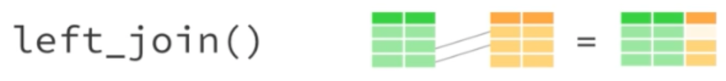
A left join returns all rows from the left table and matching rows from the right table. If there is no match in the right table, the result will have NA values for the columns from the right table. This is useful when you want to preserve all records from one dataset while adding information from another.

In ecological research, left joins are commonly used when you want to maintain all your primary data points (e.g., all species in your survey) while adding supplementary information that might not be available for every species.

df_genes_expr_left <- left_join(df_genes, df_expression, by = "gene_id")
df_genes_expr_left

# A tibble: 10 × 7
   gene_id gene_name                                  chromosome function_category    species         expression_level tissue
   <chr>   <chr>                                           <dbl> <chr>                <chr>                      <dbl> <chr> 
 1 FOXP2   Forkhead Box P2                                     7 Transcription factor Homo sapiens                15.2 Brain 
 2 FOXP2   Forkhead Box P2                                     7 Transcription factor Pan troglodytes             12.1 Brain 
 3 FOXP2   Forkhead Box P2                                     7 Transcription factor Mus musculus                 9.8 Brain 
 4 BRCA1   Breast Cancer 1                                    17 Tumor suppressor     Homo sapiens                22.5 Breast
 5 BRCA1   Breast Cancer 1                                    17 Tumor suppressor     Mus musculus                18.7 Breast
 6 CFTR    Cystic Fibrosis Transmembrane Conductor             7 Ion channel          NA                          NA   NA    
 7 MC1R    Melanocortin 1 Receptor                            16 Receptor             Homo sapiens                 8.9 Skin  
 8 MC1R    Melanocortin 1 Receptor                            16 Receptor             Canis lupus                 14.3 Skin  
 9 OCA2    Oculocutaneous Albinism II                         15 Transport protein    Homo sapiens                 5.6 Eye   
10 HERC2   HECT and RLD Domain Containing E3 Ligase 2         15 E3 ubiquitin ligase  Homo sapiens                11.2 Eye  

In this example, we’re performing a left join between df_genes (left table) and df_expression (right table). The result includes all genes from df_genes, even those without expression data. Notice that CFTR is included in the result, but with NA values for the expression-related columns because there is no matching CFTR record in the df_expression table.

Left joins are particularly useful in evolutionary biology when you want to retain all the species or genes in your primary dataset, regardless of whether they have corresponding data in secondary datasets. This helps avoid inadvertently filtering out important data points due to missing information.

Full/Outer Joins

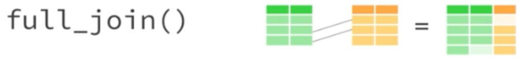
A full join (also called outer join) returns all rows from both tables, regardless of whether there are matches. When there is no match, the result will have NA values for the columns from the table without a matching record. This is useful when you want to ensure you’re not missing any data from either table.

In biodiversity research, full joins can be valuable when combining datasets from different sources to create a comprehensive database that doesn’t exclude any records from either source.

df_genes_cons_full <- full_join(df_genes, df_conservation, by = "gene_id")
df_genes_cons_full

# A tibble: 8 × 7
  gene_id gene_name                                  chromosome function_category    conservation_score last_common_ancestor millions_years_ago
  <chr>   <chr>                                           <dbl> <chr>                             <dbl> <chr>                             <dbl>
1 FOXP2   Forkhead Box P2                                     7 Transcription factor               0.92 Amniotes                            312
2 BRCA1   Breast Cancer 1                                    17 Tumor suppressor                   0.88 Mammals                             125
3 CFTR    Cystic Fibrosis Transmembrane Conductor             7 Ion channel                        0.85 Mammals                             125
4 MC1R    Melanocortin 1 Receptor                            16 Receptor                           0.76 Vertebrates                         500
5 OCA2    Oculocutaneous Albinism II                         15 Transport protein                  0.81 Vertebrates                         500
6 HERC2   HECT and RLD Domain Containing E3 Ligase 2         15 E3 ubiquitin ligase               NA    NA                                   NA
7 SLC24A5 NA                                                 NA NA                                 0.74 Vertebrates                         500
8 TYR     NA                                                 NA NA                                 0.79 Vertebrates                         500

In this example, we’re performing a full join between df_genes and df_conservation. The result includes all genes from both tables. Notice that:

• SLC24A5 and TYR from df_conservation are included but have NA values for the gene information columns because they don’t appear in df_genes
• HERC2 from df_genes is included but has NA values for the conservation-related columns because it doesn’t appear in df_conservation
• Genes that appear in both tables (FOXP2, BRCA1, CFTR, MC1R, OCA2) have complete information from both sources

Full joins are particularly useful when creating comprehensive datasets that combine information from multiple sources, ensuring no records are inadvertently excluded due to missing matches.

A real-life example – the Baxter dataset

Now let’s explore a real-life example from microbiome research using the Baxter colorectal cancer dataset. This dataset comes from a study examining the relationship between gut microbiome composition and colorectal cancer. It consists of three related tables:

• Metadata (df_metadata): Contains information about patient samples, including their disease status
• OTU counts (df_otu): Contains the abundance of each Operational Taxonomic Unit (OTU, a group of related bacterial sequences) in each sample
• Taxonomy (df_taxa): Contains the taxonomic classification of each OTU (kingdom, phylum, class, order, family, genus)

This is a common structure in microbiome studies, where the data is spread across multiple tables that need to be combined for comprehensive analysis.

Let’s load in the data. Some preliminary cleaning will be done which is not the focus of this article.

df_metadata <- read_tsv(
  "https://raw.githubusercontent.com/riffomonas/minimalR-raw_data/refs/heads/master/baxter.metadata.tsv",
  col_types = cols(
    sample = col_character(),
    Dx_Bin = col_character()
  )
) %>%
  select(sample, Dx_Bin) %>%
  rename(disease_status = Dx_Bin) %>%
  drop_na(disease_status) %>% # Drop rows with NA disease status
  mutate(
    disease_status = fct_relevel(disease_status, c("Normal", "High Risk Normal", "Adenoma", "Adv Adenoma", "Cancer"))
  )
df_metadata

# A tibble: 490 × 2
   sample  disease_status  
   <chr>   <fct>           
 1 2003650 High Risk Normal
 2 2005650 High Risk Normal
 3 2007660 High Risk Normal
 4 2009650 Adenoma         
 5 2013660 Normal          
 6 2015650 High Risk Normal
 7 2017660 Cancer          
 8 2019651 Normal          
 9 2023680 High Risk Normal
10 2025653 Cancer          
# ℹ 480 more rows

df_otu <- read_tsv(
  "https://raw.githubusercontent.com/riffomonas/minimalR-raw_data/refs/heads/master/baxter.subsample.shared",
  col_types = cols(
    Group = col_character(),
    .default = col_double()
  )
) %>%
  select(Group, starts_with("Otu")) %>%
  rename(sample = Group) %>% # This will be used to join with the metadata
  pivot_longer(cols = starts_with("Otu"), names_to = "otu", values_to = "count")
df_otu

# A tibble: 2,683,240 × 3
   sample  otu       count
   <chr>   <chr>     <dbl>
 1 2003650 Otu000001   346
 2 2003650 Otu000002   267
 3 2003650 Otu000003   289
 4 2003650 Otu000004   243
 5 2003650 Otu000005   263
 6 2003650 Otu000006   681
 7 2003650 Otu000007   244
 8 2003650 Otu000008    88
 9 2003650 Otu000009   108
10 2003650 Otu000010   253
# ℹ 2,683,230 more rows

df_taxa <- read_tsv(
  "https://raw.githubusercontent.com/riffomonas/minimalR-raw_data/refs/heads/master/baxter.cons.taxonomy"
) %>%
  select(OTU, Taxonomy) %>%
  rename(
    otu = OTU, # This will be used to join with the OTU counts
    taxonomy = Taxonomy
  ) %>%
  mutate(
    taxonomy = str_replace_all(taxonomy, "\\(\\d+\\)", ""), # Remove bracketed numbers
    taxonomy = str_replace_all(taxonomy, "unclassified", "NA"), # Replace unclassified with "NA" will become R's NA
    taxonomy = str_replace_all(taxonomy, ";$", "") # Remove trailing semicolon
  ) %>%
  # Separate the taxonomy into separate columns via the ";" delimiter
  separate(
    taxonomy,
    into = c("kingdom", "phylum", "class", "order", "family", "genus"),
    sep = ";",
    remove = TRUE, # Remove the original taxonomy column
    convert = TRUE # Convert "NA" to NA
  )
df_taxa

# A tibble: 9,467 × 7
   otu       kingdom  phylum          class            order              family              genus           
   <chr>     <chr>    <chr>           <chr>            <chr>              <chr>               <chr>           
 1 Otu000001 Bacteria Firmicutes      Clostridia       Clostridiales      Lachnospiraceae     Blautia         
 2 Otu000002 Bacteria Bacteroidetes   Bacteroidia      Bacteroidales      Bacteroidaceae      Bacteroides     
 3 Otu000003 Bacteria Bacteroidetes   Bacteroidia      Bacteroidales      Bacteroidaceae      Bacteroides     
 4 Otu000004 Bacteria Verrucomicrobia Verrucomicrobiae Verrucomicrobiales Verrucomicrobiaceae Akkermansia     
 5 Otu000005 Bacteria Firmicutes      Clostridia       Clostridiales      Lachnospiraceae     Roseburia       
 6 Otu000006 Bacteria Firmicutes      Clostridia       Clostridiales      Ruminococcaceae     Faecalibacterium
 7 Otu000007 Bacteria Bacteroidetes   Bacteroidia      Bacteroidales      Bacteroidaceae      Bacteroides     
 8 Otu000008 Bacteria Firmicutes      Clostridia       Clostridiales      Lachnospiraceae     Anaerostipes    
 9 Otu000009 Bacteria Firmicutes      Clostridia       Clostridiales      Lachnospiraceae     Blautia         
10 Otu000010 Bacteria Firmicutes      Clostridia       Clostridiales      NA                  NA              
# ℹ 9,457 more rows

Association Tables

In relational database design, an association table (sometimes called a junction table or bridge table) connects two or more tables in a many-to-many relationship. In our Baxter dataset, the OTU table (df_otu) functions as an association table that connects samples to taxa.

The df_otu table contains two key columns:

• sample: Links to the metadata table (df_metadata)
• otu: Links to the taxonomy table (df_taxa)

This structure is common in ecological datasets, where the association table records the abundance or presence/absence of each taxon in each sampling unit. It allows for a many-to-many relationship: each sample contains multiple OTUs, and each OTU can be found in multiple samples.

Joining the Tables

To analyze the relationship between microbiome composition and disease status, we need to combine all three tables. We’ll use inner joins to connect the tables based on their shared columns:

• First join df_otu with df_taxa using the otu column
• Then join the result with df_metadata using the sample column

df_combined <- df_otu %>%
  inner_join(df_taxa, by = "otu") %>%
  inner_join(df_metadata, by = "sample")
df_combined

# A tibble: 2,683,240 × 10
   sample  otu       count kingdom  phylum          class            order              family              genus            disease_status  
   <chr>   <chr>     <dbl> <chr>    <chr>           <chr>            <chr>              <chr>               <chr>            <fct>           
 1 2003650 Otu000001   346 Bacteria Firmicutes      Clostridia       Clostridiales      Lachnospiraceae     Blautia          High Risk Normal
 2 2003650 Otu000002   267 Bacteria Bacteroidetes   Bacteroidia      Bacteroidales      Bacteroidaceae      Bacteroides      High Risk Normal
 3 2003650 Otu000003   289 Bacteria Bacteroidetes   Bacteroidia      Bacteroidales      Bacteroidaceae      Bacteroides      High Risk Normal
 4 2003650 Otu000004   243 Bacteria Verrucomicrobia Verrucomicrobiae Verrucomicrobiales Verrucomicrobiaceae Akkermansia      High Risk Normal
 5 2003650 Otu000005   263 Bacteria Firmicutes      Clostridia       Clostridiales      Lachnospiraceae     Roseburia        High Risk Normal
 6 2003650 Otu000006   681 Bacteria Firmicutes      Clostridia       Clostridiales      Ruminococcaceae     Faecalibacterium High Risk Normal
 7 2003650 Otu000007   244 Bacteria Bacteroidetes   Bacteroidia      Bacteroidales      Bacteroidaceae      Bacteroides      High Risk Normal
 8 2003650 Otu000008    88 Bacteria Firmicutes      Clostridia       Clostridiales      Lachnospiraceae     Anaerostipes     High Risk Normal
 9 2003650 Otu000009   108 Bacteria Firmicutes      Clostridia       Clostridiales      Lachnospiraceae     Blautia          High Risk Normal
10 2003650 Otu000010   253 Bacteria Firmicutes      Clostridia       Clostridiales      NA                  NA               High Risk Normal
# ℹ 2,683,230 more rows

The resulting df_combined table now contains all the information we need for our analysis:

• Sample information (sample ID and disease status)
• OTU counts (abundance of each bacterial group)
• Taxonomic classification of each OTU

With this combined dataset, we can now analyze patterns in bacterial community composition across different disease states, identify taxonomic groups that may be associated with colorectal cancer, and perform various statistical analyses to test specific hypotheses.

This example demonstrates the power of joining tables to integrate different types of biological data. By combining sample metadata, abundance data, and taxonomic information, we can address complex ecological questions that would be impossible to answer with any single table alone.

Summary

Understanding how to join tables is essential for working with complex biological datasets that span multiple levels of organization. In this article, we’ve explored:

• Inner joins: Combine tables based on matching records, useful when you need complete information from both sources
• Left joins: Keep all records from one table while adding matching information from another, useful for preserving your primary dataset
• Full joins: Retain all records from both tables, useful for creating comprehensive datasets
• Association tables: Bridge between different entities in a many-to-many relationship, common in ecological data

These techniques have wide-ranging applications in ecology and evolutionary biology:

• Integrating genetic data with phenotypic measurements
• Combining taxonomic information with abundance data
• Linking spatial data with environmental measurements
• Analyzing temporal patterns across multiple datasets

By mastering these relational data concepts, you’ll be better equipped to handle the complex, multidimensional datasets that are increasingly common in modern biological research. Rather than being limited to analyzing isolated datasets, you can integrate information from multiple sources to address more sophisticated research questions and gain deeper insights into ecological and evolutionary processes.