Filtering & Subsetting Data
Filtering or subsetting data means selecting a portion of a dataset (like a dataframe) based on specific criteria. A common task is creating a new dataframe by choosing rows from an existing one based on values in one or more columns.
This tutorial demonstrates how to perform these tasks using both base R functions and functions from the Tidyverse.
Pie Crabs Dataset
First, we need to load the necessary libraries and the example dataset. We’ll be using the pie_crab dataset from the lterdatasampler package and functions from the tidyverse package.
library(tidyverse) # Automatically loads dlpyr as well
library(lterdatasampler) # For the example dataset

# Load the crabs dataset
crabs <- lterdatasampler::pie_crab
str(crabs)
## tibble [392 × 9] (S3: tbl_df/tbl/data.frame)
## $ date : Date[1:392], format: "2016-07-24" "2016-07-24" ...
## $ latitude : num [1:392] 30 30 30 30 ...
## $ site : chr [1:392] "GTM" "GTM" "GTM" "GTM" ...
## $ size : num [1:392] 12.4 14.2 14.5 12.9 ...
## $ air_temp : num [1:392] 21.8 21.8 21.8 21.8 ...
## $ air_temp_sd : num [1:392] 6.39 6.39 6.39 6.39 ...
## $ water_temp : num [1:392] 24.5 24.5 24.5 24.5 ...
## $ water_temp_sd: num [1:392] 6.12 6.12 6.12 6.12 ...
## $ name : chr [1:392] "Guana Tolomoto Matanzas NERR" "Guana Tolomoto Matanzas NERR" ...The str(crabs) output shows us the structure of the crabs dataframe. It has 392 observations and 9 variables, including site (character) and size (numeric), which we will use in our filtering examples.
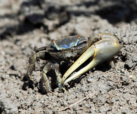
Fiddler Crabs
The Atlantic marsh fiddler crab (Minuca pugnax) is found along the Eastern seaboard of the United States. The data in our example dataset comes from the Plum Island Long Term Ecological Research Site in Massachusetts.
Filter Based on a Single Condition
We often want to select rows based on the value of a specific column. For this, we use logical operators. Common operators include:
==(equal to)!=(not equal to)>(greater than)<(less than)>=(greater than or equal to)<=(less than or equal to)%in%(value is in a set of specified values)!(negation, used with other logical expressions like!is.na())is.na()(checks if a value isNA)
Let’s select rows where the site is “GTM”.
Base R
In base R, you can use bracket indexing [row_condition, column_selection] or the subset() function.
# Base R - via bracket indexing
crabs[crabs$site == "GTM", ]

# Base R - via subset() function
subset(crabs, site == "GTM")
Tidyverse
The Tidyverse approach uses the filter() function from the dplyr package.
# Tidyverse
crabs %>% filter(site == "GTM")
The Boolean Vector Concept
The condition inside the brackets (e.g., crabs$site == "GTM") creates a logical vector (a series of TRUE/FALSE values). Rows where the condition is TRUE are kept. You can store this logical vector in a variable and use it for filtering.
boolean_mask <- crabs$site == "GTM"
# head(boolean_mask) # This would show TRUE/FALSE values

# Base R - via bracket indexing with a boolean vector
crabs[boolean_mask, ]

# Base R - via subset() function with a boolean vector
subset(crabs, boolean_mask)

# Tidyverse - filter() also accepts boolean vectors
crabs %>% filter(boolean_mask)
Filter Based on the %in% Operator
To select rows where a column’s value matches any of several specified values, use the %in% operator. Let’s select crabs from sites “GTM”, “SI”, or “NIB”.
selected_sites <- c("GTM", "SI", "NIB")

# Base R - via bracket indexing
crabs[crabs$site %in% selected_sites, ]

# Base R - via subset() function
subset(crabs, site %in% selected_sites)

# Tidyverse
crabs %>% filter(site %in% selected_sites)
Removing NAs
Missing values (NA) can be problematic. We’ll use the ntl_icecover dataset, which is known to have NAs, to demonstrate how to remove rows with NAs in a specific column.
ice_data <- lterdatasampler::ntl_icecover
head(ice_data)
# A tibble: 6 × 5
lakeid ice_on ice_off ice_duration year
<fct> <date> <date> <dbl> <dbl>
1 Lake Mendota NA 1853-04-05 NA 1852
2 Lake Mendota 1853-12-27 NA NA 1853
3 Lake Mendota 1855-12-18 1856-04-14 118 1855
4 Lake Mendota 1856-12-06 1857-05-06 151 1856
5 Lake Mendota 1857-11-25 1858-03-26 121 1857
6 Lake Mendota 1858-12-08 1859-03-14 96 1858Our goal is to remove rows where ice_duration is NA.

Ice Cover Data
This dataset contains information about ice cover duration for lakes near Madison, WI, USA, used for monitoring climate change effects.
Base R
Use !is.na() to select rows where ice_duration is NOT NA.
# Base R - Using !is.na()
ice_data_no_na_base <- ice_data[!is.na(ice_data$ice_duration), ]
head(ice_data_no_na_base)
Tidyverse
In Tidyverse, you can use filter(!is.na(column)) or the convenient drop_na(column) function.
# Tidyverse - Using filter()
ice_data_no_na_tidy_filter <- ice_data %>% filter(!is.na(ice_duration))
head(ice_data_no_na_tidy_filter)

# Tidyverse - Using drop_na()
ice_data_no_na_tidy_drop <- ice_data %>% drop_na(ice_duration)
head(ice_data_no_na_tidy_drop)
Filter Based on Multiple Conditions
You can combine conditions using logical combinators:
&(AND: both conditions must be true)|(OR: at least one condition must be true)xor()(Exclusive OR: only one condition can be true)
Let’s go back to the crabs dataset.
AND Condition
Goal: Select rows where site is “GTM” AND size is greater than 15mm.
# Base R - via bracket indexing
crabs[crabs$site == "GTM" & crabs$size > 15, ]

# Base R - via subset() function
subset(crabs, site == "GTM" & size > 15)

# Tidyverse - using &
crabs %>% filter(site == "GTM" & size > 15)

# Tidyverse - using multiple arguments in filter() (implicit AND)
crabs %>% filter(site == "GTM", size > 15)
OR Condition
Goal: Select rows where site is “GTM” OR size is greater than 25mm.
# Base R - via bracket indexing
crabs[crabs$site == "GTM" | crabs$size > 25, ]

# Base R - via subset() function
subset(crabs, site == "GTM" | size > 25)

# Tidyverse
crabs %>% filter(site == "GTM" | size > 25)
Filtering by Known Numeric Indices
You can select rows based on their position (row number).
Select First/Specific/Last Rows
# Goal: Select the first 3 rows
# Base R
crabs[1:3, ]
# Tidyverse
crabs %>% slice(1:3)

# Goal: Select the 1st, 5th, and 10th rows
# Base R
crabs[c(1, 5, 10), ]
# Tidyverse
crabs %>% slice(c(1, 5, 10))

# Goal: Select the last 3 rows
# Base R
crabs[(nrow(crabs) - 2):nrow(crabs), ]
# Tidyverse
# n() gives the current group size (here, total rows)
crabs %>% slice((n() - 2):n())
Removing Duplicate Rows
Sometimes datasets contain duplicate rows. You can remove them based on all columns or a subset of columns.
Remove Duplicates Across All Columns
# For comparison
crabs %>% nrow()

# Base R - via unique()
crabs %>% unique() %>% nrow()

# Tidyverse - via distinct()
crabs %>% distinct() %>% nrow()
Keep Distinct Rows Based on Specific Columns
This is useful if you want to keep the first occurrence of unique values in certain columns.
# Goal: Keep only distinct rows based on the 'date' column
# Base R
# !duplicated() returns TRUE for the first occurrence
crabs[!duplicated(crabs$date), ] %>% head()

# Tidyverse
# .keep_all = TRUE ensures all columns are retained for the distinct rows
crabs %>% distinct(date, .keep_all = TRUE) %>% head()
Other Beneficial Concepts
The dplyr package offers many other useful functions. For example, between() can select rows where a numeric value falls within a specified range.
Filtering a Numeric Range with between()
Goal: Select crabs with size between 10mm and 12mm (inclusive), excluding NAs in size.
# Base R
crabs[crabs$size >= 10 & crabs$size <= 12 & !is.na(crabs$size), ] %>% summary()

# Tidyverse
# The between() function is inclusive by default.
# It also handles NAs correctly (NA & NA results in NA, which filter drops).
crabs %>% filter(between(size, 10, 12)) %>% summary()
As you become more familiar with these functions, you’ll find you can combine them in many ways to precisely subset and filter your data for analysis. Remember to check your results at each step, especially when working with complex conditions.