Grouping & Summarizing Data in R
Often in data analysis, we need to calculate summary statistics for different groups within our dataset. For example, we might want to find the average weight of animals based on their sex, or the total count of observations per year. The dplyr package, part of the Tidyverse, provides powerful and intuitive tools for these tasks, primarily through the group_by() and summarise() (or summarize()) functions. This article will guide you through various ways to group and summarize your data effectively.
Setup & Initial Data Inspection
First, let’s load the necessary libraries and our example dataset. We’ll be using the knz_bison dataset from the lterdatasampler package, which contains data on bison from the Konza Prairie LTER site. We’ll also create an approx_age column by subtracting the animal’s year of birth (animal_yob) from the recording year (rec_year).
# --- 0. Setup & Initial Data Inspection --- #
library(lterdatasampler)
library(tidyverse)

bison_data <- lterdatasampler::knz_bison %>%
  mutate(approx_age = rec_year - animal_yob)

bison_data
# A tibble: 8,325 × 9
data_code rec_year rec_month rec_day animal_code animal_sex animal_weight animal_yob approx_age
<chr> <dbl> <dbl> <dbl> <chr> <chr> <dbl> <dbl> <dbl>
1 CBH01 1994 11 8 813 F 890 1981 13
2 CBH01 1994 11 8 834 F 1074 1983 11
3 CBH01 1994 11 8 B-301 F 1060 1983 11
4 CBH01 1994 11 8 B-402 F 989 1984 10
5 CBH01 1994 11 8 B-403 F 1062 1984 10
6 CBH01 1994 11 8 B-502 F 978 1985 9
7 CBH01 1994 11 8 B-503 F 1068 1985 9
8 CBH01 1994 11 8 B-504 F 1024 1985 9
9 CBH01 1994 11 8 B-601 F 978 1986 8
10 CBH01 1994 11 8 B-602 F 1188 1986 8
# ℹ 8,315 more rows
# ℹ Use `print(n = ...)` to see more rowsPlains Bison at Konza Prairie
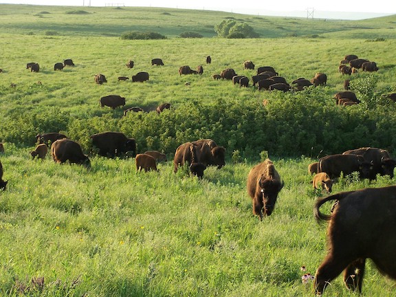
The data used in these examples come from long-term studies of Plains bison (Bison bison bison) at the Konza Prairie Biological Station, an NSF Long-Term Ecological Research (LTER) site in northeastern Kansas. Understanding population dynamics, such as sex ratios and age structures across years, is crucial for managing these iconic prairie animals and their grassland ecosystem.
Basic Grouping & Summarizing
The core idea is to first group the data by one or more variables using group_by(), and then apply summary functions using summarise(). The summarise() function creates a new data frame containing one row for each group, with new columns representing the summary statistics.
Group by One Variable
When working within summarise(), you have access to several helpful context-dependent functions. A commonly used one is n(), which returns the number of rows (observations) in the current group. Another useful one is n_distinct(variable_name), which counts the number of unique values of a specified variable within the current group. In this example, we will use n() to count observations.
Let’s group the bison data by animal_sex and calculate the mean weight, standard deviation of weight, and the number of observations for each sex using the aforementioned n() helper function. Note also the use of na.rm = TRUE within mean() and sd() to ensure that missing values (NA) in the animal_weight column are ignored during calculations.
# Example: Group by one variable ('animal_sex') and calculate mean weight,
# standard deviation of weight, and count of observations.
bison_data %>%
  group_by(animal_sex) %>%
  summarise(
    mean_weight = mean(animal_weight, na.rm = TRUE),
    sd_weight = sd(animal_weight, na.rm = TRUE),
    n_obs = n()
  )
# A tibble: 2 × 4
animal_sex mean_weight sd_weight n_obs
<chr> <dbl> <dbl> <int>
1 F 762. 282. 5285
2 M 728. 420. 3040The output shows that we have 5285 female (F) bison with a mean weight of approximately 762 units, and 3040 male (M) bison with a mean weight of approximately 728 units.
Group by Multiple Variables
We can also group by multiple variables. For instance, let’s calculate the mean weight of bison grouped by both rec_year (recording year) and animal_sex.
# Example: Group by multiple variables ('rec_year', 'animal_sex')
# and calculate mean weight.
bison_data %>%
  group_by(rec_year, animal_sex) %>%
  summarise(mean_weight = mean(animal_weight, na.rm = TRUE))
# A tibble: 52 × 3
# Groups: rec_year [26]
rec_year animal_sex mean_weight
<dbl> <chr> <dbl>
1 1994 F 700.
2 1994 M 532.
3 1995 F 826.
4 1995 M 812.
5 1996 F 733.
6 1996 M 696.
# ... (output truncated for brevity, showing first 6 rows, see R script for full output)This provides a more granular view, showing how mean weight varies by sex within each year. Notice the output indicates # Groups: rec_year [26]. This means that after the summarise() operation, the resulting tibble is still grouped by the first grouping variable, rec_year. This can be important for subsequent operations. We’ll discuss how to manage this next.
Controlling Grouping Structure after summarise()
When you use summarise() on data grouped by multiple variables, it peels off one layer of grouping by default. For example, if you group_by(var1, var2) and then summarise(), the result will be grouped by var1. You can control this behavior with the .groups argument in summarise() or by using ungroup().
.groups = "drop_last": (Default) Peels off the last grouping variable..groups = "drop": Drops all grouping levels. Equivalent to callingungroup()afterwards..groups = "keep": Keeps the same grouping structure as the input..groups = "rowwise": Treats each row as a group. (Less common withsummarise).
Using ungroup()
If you want to perform further operations on the summarized data that should not be group-wise, you can explicitly remove all grouping with ungroup(). In this example, after calculating mean weight per year and sex, we ungroup() and then calculate an overall mean weight across these summarized values.
# Example: Using ungroup().
# Useful if you want to perform further operations that shouldn't be group-wise.
bison_data %>%
  group_by(rec_year, animal_sex) %>%
  summarise(
    mean_weight = mean(animal_weight, na.rm = TRUE),
    .groups = "drop" # Alternatively, you can use ungroup() after summarise()
  ) %>%
  # Without ungroup() or .groups = "drop",
  # the mutate() would be applied to each group of rec_year separately
  mutate(
    overall_mean_weight = mean(mean_weight, na.rm = TRUE)
  )
# A tibble: 52 × 4
rec_year animal_sex mean_weight overall_mean_weight
<dbl> <chr> <dbl> <dbl>
1 1994 F 700. 739.
2 1994 M 532. 739.
3 1995 F 826. 739.
4 1995 M 812. 739.
5 1996 F 733. 739.
6 1996 M 696. 739.
# ... (output truncated for brevity, see R script for full output)Here, setting .groups = "drop" in summarise() achieves the same as piping to ungroup(). If we had omitted this or ungroup(), the mutate() for overall_mean_weight would have calculated the mean of mean_weight *within each rec_year* (because the data would still be grouped by rec_year), which is not what we intended here.
Multiple Summary Statistics & Columns with summarise() and across()
The across() function is a powerful tool to apply the same transformation or summary function(s) to multiple columns. It’s often used within summarise() or mutate().
Using across() to Apply One Summary Function to Multiple Columns
Let’s calculate the mean of both animal_weight and our newly created approx_age, grouped by animal_sex.
A key feature of across() is the .names argument, which allows you to control the names of the output columns. It uses a template string where:
{.col}refers to the original column name being processed.{.fn}refers to the name of the function being applied (useful when applying multiple functions, see next example).
In this example, .names = "mean_{.col}" will create columns like mean_animal_weight and mean_approx_age.
# Example: Using across() to apply one summary function to multiple columns.
# Calculate mean of 'animal_weight' and 'approx_age' by 'animal_sex'.
bison_data %>%
  group_by(animal_sex) %>%
  summarise(across(
    .cols = c(animal_weight, approx_age),
    .fns = mean,
    # Other arguments to pass to the function being applied (mean)
    na.rm = TRUE,
    # .names controls output column names
    .names = "mean_{.col}"
  ))
# A tibble: 2 × 3
animal_sex mean_animal_weight mean_approx_age
<chr> <dbl> <dbl>
1 F 762. 4.55
2 M 728. 1.65Using across() to Apply Multiple Summary Functions to Multiple Columns
You can also apply a list of functions with across(). Here, we calculate both the mean (named avg) and standard deviation (named stdev) for animal_weight and approx_age, grouped by animal_sex. We use the purrr-style lambda function syntax (e.g., ~ mean(., na.rm = TRUE)), where . represents the column data being passed to the function.
The .names argument now uses both {.col} for the original column name and {.fn} for the name of the function from our list (avg or stdev). So, .names = "{.col}_{.fn}" will generate names like animal_weight_avg, animal_weight_stdev, etc.
# Example: Using across() to apply multiple summary functions to multiple columns.
# Calculate mean and sd for 'animal_weight' and 'approx_age' by 'animal_sex'.
bison_data %>%
  group_by(animal_sex) %>%
  summarise(across(
    .cols = c(animal_weight, approx_age),
    .fns = list(
      avg = ~ mean(., na.rm = TRUE),
      stdev = ~ sd(., na.rm = TRUE)
    ),
    # .names controls output column names
    # .fn is the function name from the list (avg, stdev)
    # .col is the original column name
    .names = "{.col}_{.fn}"
  ))
# A tibble: 2 × 5
animal_sex animal_weight_avg animal_weight_stdev approx_age_avg approx_age_stdev
<chr> <dbl> <dbl> <dbl> <dbl>
1 F 762. 282. 4.55 4.52
2 M 728. 420. 1.65 1.88Advanced Summaries
Proportional Composition
Grouping and summarizing can be chained for more complex analyses. Let’s tackle a common scenario: calculating the proportional composition of subgroups. Our goal is to find, for each recording year, the percentage of male and female bison, such that within each year, these percentages sum to 100%.
The strategy involves several steps:
- Filter out any rows where
approx_ageoranimal_sexis missing, as these are crucial for our calculation. - Group by
rec_yearandanimal_sex. - Count the number of bison in each group (
count_in_year = n()). We use.groups = "drop"here to remove all grouping after this initial summary, making the next step simpler. (Alternatively, one could use.groups = "drop_last"orungroup() %>% group_by(rec_year)). - Re-group by just
rec_year. - Within each year, calculate the total number of bison for that year (
total_for_year = sum(count_in_year)). - Calculate the percentage for each sex within that year:
(count_in_year / total_for_year) * 100. ungroup()for a clean final tibble andarrange()for readability.
# Example: Calculating Proportional Composition within Subgroups
# Goal: For each recording year, calculate the male and female percentage of bison for that year
# Therefore each year's percentages should sum to 100%

bison_sex_pct_by_year <- bison_data %>%
  filter(!is.na(approx_age) & !is.na(animal_sex)) %>% # Ensure age and sex are available
  group_by(rec_year, animal_sex) %>%
  summarise(count_in_year = n(), .groups = "drop") %>% # Count per sex per year, then drop all groups
  group_by(rec_year) %>% # Re-group by year to sum counts within each year
  mutate(
    total_for_year = sum(count_in_year),
    percentage_of_sex_in_year = (count_in_year / total_for_year) * 100
  ) %>%
  ungroup() %>% # Remove grouping
  arrange(rec_year, animal_sex) # Order for easier viewing

bison_sex_pct_by_year
# A tibble: 52 × 5
rec_year animal_sex count_in_year total_for_year percentage_of_sex_in_year
<dbl> <chr> <int> <int> <dbl>
1 1994 F 78 144 54.2
2 1994 M 66 144 45.8
3 1995 F 71 136 52.2
4 1995 M 65 136 47.8
5 1996 F 114 193 59.1
6 1996 M 79 193 40.9
# ... (output truncated for brevity, see R script for full output)To verify our calculation, we can group the resulting bison_sex_pct_by_year data frame by rec_year and sum the percentage_of_sex_in_year. Each year should sum to 100%.
# Verification: The total percentage for each year should be 100
bison_sex_pct_by_year %>%
  group_by(rec_year) %>%
  summarise(total_percentage = sum(percentage_of_sex_in_year), .groups = "drop")
# A tibble: 26 × 2
rec_year total_percentage
<dbl> <dbl>
1 1994 100
2 1995 100
3 1996 100
4 1997 100
5 1998 100
6 1999 100
# ... (output truncated for brevity, see R script for full output)The verification confirms our method is correct, with each year’s percentages summing to 100 (allowing for minor floating-point inaccuracies if they were to occur, though not visible here).
Conclusion
The group_by() and summarise() functions, especially when combined with across(), provide a flexible and powerful framework for data aggregation and summary in R. By understanding how to group by single or multiple variables, control grouping structures, and apply various summary functions, you can efficiently derive meaningful insights from your datasets. Remember to consider how NA values are handled (e.g., using na.rm = TRUE) and how the grouping structure persists or is modified after summarization to ensure your analyses are accurate and lead to the intended results.