Creating & Mutating Columns
A fundamental part of data wrangling is creating new columns or modifying (mutating) existing ones. New columns can hold constant values, results of calculations between existing columns, or categorical variables derived from other data. This tutorial explores how to perform these operations in R, contrasting base R methods with the more expressive and often more readable functions from the dplyr package, part of the Tidyverse.
Setup: Loading Data and Libraries
We begin by loading the tidyverse (which includes dplyr) for its data manipulation tools and lterdatasampler for our example dataset.
library(tidyverse)
library(lterdatasampler)
We’ll use the hbr_maples dataset, which contains data on sugar maple seedlings from the Hubbard Brook Experimental Forest. Let’s load it and inspect its structure.
maples <- lterdatasampler::hbr_maples
str(maples)
tibble [359 × 11] (S3: tbl_df/tbl/data.frame)
$ year : num [1:359] 2003 2003 2003 2003 2003 ...
$ watershed : Factor w/ 2 levels "Reference","W1": 1 1 1 1 1 1 1 1 1 1 ...
$ elevation : Factor w/ 2 levels "Low","Mid": 1 1 1 1 1 1 1 1 1 1 ...
$ transect : Factor w/ 12 levels "R1","R2","R3",..: 1 1 1 1 1 1 1 1 1 1 ...
$ sample : Factor w/ 20 levels "1","2","3","4",..: 1 2 3 4 5 6 7 8 9 10 ...
$ stem_length : num [1:359] 86.9 114 83.5 68.1 72.1 77.7 85.5 81.6 92.9 59.6 ...
$ leaf1area : num [1:359] 13.84 14.57 12.45 9.97 6.84 ...
$ leaf2area : num [1:359] 12.13 15.27 9.73 10.07 5.48 ...
$ leaf_dry_mass : num [1:359] 0.0453 0.0476 0.0423 0.0397 0.0204 0.0317 0.0382 0.0179 0.0286 0.0125 ...
$ stem_dry_mass : num [1:359] 0.03 0.0338 0.0248 0.0194 0.018 0.0246 0.0316 0.015 0.0291 0.0149 ...
$ corrected_leaf_area: num [1:359] 29.1 33 25.3 23.2 15.5 ...To make our examples clearer and less verbose, we’ll select a subset of these columns to work with, calling it maples_sub.
maples_sub <- maples %>%
  select(year, watershed, elevation, stem_length, leaf1area, leaf2area, corrected_leaf_area)

head(maples_sub)
# A tibble: 6 × 7
year watershed elevation stem_length leaf1area leaf2area corrected_leaf_area
<dbl> <fct> <fct> <dbl> <dbl> <dbl> <dbl>
1 2003 Reference Low 86.9 13.8 12.1 29.1
2 2003 Reference Low 114 14.6 15.3 33.0
3 2003 Reference Low 83.5 12.5 9.73 25.3
4 2003 Reference Low 68.1 9.97 10.1 23.2
5 2003 Reference Low 72.1 6.84 5.48 15.5
6 2003 Reference Low 77.7 9.66 7.64 20.4Sugar Maple Seedlings at Hubbard Brook
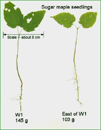
The sugar maple (Acer saccharum) is a key species in northeastern North American forests, famous for maple syrup. Data from long-term research sites like Hubbard Brook Experimental Forest in New Hampshire help scientists understand factors affecting their growth and survival, such as soil acidification from acid rain.
Creating Columns
This section demonstrates how to add entirely new columns to your dataframe.
Base R
In base R, you typically create a new column using the $ operator followed by the new column name and assign values to it.
# Create a copy for base R examples to avoid altering maples_sub
maples_base_create <- maples_sub

# Example: Adding a new column with a single, constant value
maples_base_create$site_name <- "Hubbard Brook"
head(maples_base_create)
# A tibble: 6 × 8
year watershed elevation stem_length leaf1area leaf2area corrected_leaf_area site_name
<dbl> <fct> <fct> <dbl> <dbl> <dbl> <dbl> <chr>
1 2003 Reference Low 86.9 13.8 12.1 29.1 Hubbard Brook
2 2003 Reference Low 114 14.6 15.3 33.0 Hubbard Brook
3 2003 Reference Low 83.5 12.5 9.73 25.3 Hubbard Brook
4 2003 Reference Low 68.1 9.97 10.1 23.2 Hubbard Brook
5 2003 Reference Low 72.1 6.84 5.48 15.5 Hubbard Brook
6 2003 Reference Low 77.7 9.66 7.64 20.4 Hubbard Brook# Example 1.2: Adding a new column based on existing columns
# Calculate total_leaf_area by summing leaf1area and leaf2area.
# If either is NA, the result for that row will be NA.
maples_base_create$total_leaf_area_simple_sum <- maples_base_create$leaf1area + maples_base_create$leaf2area
head(maples_base_create)# A tibble: 6 × 9
year watershed elevation stem_length leaf1area leaf2area corrected_leaf_area site_name total_leaf_area_simple_sum
<dbl> <fct> <fct> <dbl> <dbl> <dbl> <dbl> <chr> <dbl>
1 2003 Reference Low 86.9 13.8 12.1 29.1 Hubbard Brook 26.0
2 2003 Reference Low 114 14.6 15.3 33.0 Hubbard Brook 29.8
3 2003 Reference Low 83.5 12.5 9.73 25.3 Hubbard Brook 22.2
4 2003 Reference Low 68.1 9.97 10.1 23.2 Hubbard Brook 20.0
5 2003 Reference Low 72.1 6.84 5.48 15.5 Hubbard Brook 12.3
6 2003 Reference Low 77.7 9.66 7.64 20.4 Hubbard Brook 17.3Tidyverse (dplyr)
The dplyr package uses the mutate() function to create new columns. mutate() is very flexible and integrates well with other dplyr verbs via the pipe %>%.
# Example: Using mutate() to add a column with a single value
maples_sub %>%
  mutate(site_name = "Hubbard Brook") %>%
  head()
# A tibble: 6 × 8
year watershed elevation stem_length leaf1area leaf2area corrected_leaf_area site_name
<dbl> <fct> <fct> <dbl> <dbl> <dbl> <dbl> <chr>
1 2003 Reference Low 86.9 13.8 12.1 29.1 Hubbard Brook
2 2003 Reference Low 114 14.6 15.3 33.0 Hubbard Brook
3 2003 Reference Low 83.5 12.5 9.73 25.3 Hubbard Brook
4 2003 Reference Low 68.1 9.97 10.1 23.2 Hubbard Brook
5 2003 Reference Low 72.1 6.84 5.48 15.5 Hubbard Brook
6 2003 Reference Low 77.7 9.66 7.64 20.4 Hubbard Brook
# Example 1.5: Using mutate() to add a new column based on existing columns
maples_sub %>%
  mutate(total_leaf_area = leaf1area + leaf2area) %>%
  head()
# A tibble: 6 × 8
year watershed elevation stem_length leaf1area leaf2area corrected_leaf_area total_leaf_area
<dbl> <fct> <fct> <dbl> <dbl> <dbl> <dbl> <dbl>
1 2003 Reference Low 86.9 13.8 12.1 29.1 26.0
2 2003 Reference Low 114 14.6 15.3 33.0 29.8
3 2003 Reference Low 83.5 12.5 9.73 25.3 22.2
4 2003 Reference Low 68.1 9.97 10.1 23.2 20.0
5 2003 Reference Low 72.1 6.84 5.48 15.5 12.3
6 2003 Reference Low 77.7 9.66 7.64 20.4 17.3Mutating Columns
Mutating columns often involves modifying existing columns or creating new columns with more complex, conditional logic based on the values in other columns.
Base R
TODO – Explain how to mutate columns in base R
# Create a fresh copy for these base R examples
maples_base_mutate <- maples_sub

# Example: Modifying an existing column by creating a new one from it
# Convert stem_length from cm to mm and store in a new column stem_length_mm.
maples_base_mutate$stem_length_mm <- maples_base_mutate$stem_length * 10
head(maples_base_mutate)
# A tibble: 6 × 8
year watershed elevation stem_length leaf1area leaf2area corrected_leaf_area stem_length_mm
<dbl> <fct> <fct> <dbl> <dbl> <dbl> <dbl> <dbl>
1 2003 Reference Low 86.9 13.8 12.1 29.1 869
2 2003 Reference Low 114 14.6 15.3 33.0 1140
3 2003 Reference Low 83.5 12.5 9.73 25.3 835
4 2003 Reference Low 68.1 9.97 10.1 23.2 681
5 2003 Reference Low 72.1 6.84 5.48 15.5 721
6 2003 Reference Low 77.7 9.66 7.64 20.4 777 TODO – Explain the use of conditional modification to create a new column
# Example: Conditional modification to create a new column
# Create stem_length_adjusted: if watershed is "W1", add 100 to stem_length, else use original stem_length.
maples_base_mutate$stem_length_adjusted <- maples_base_mutate$stem_length # Initialize
w1_indices <- maples_base_mutate$watershed == "W1" & !is.na(maples_base_mutate$stem_length)
maples_base_mutate$stem_length_adjusted[w1_indices] <- maples_base_mutate$stem_length[w1_indices] + 100
head(maples_base_mutate %>% select(watershed, stem_length, stem_length_adjusted))
# A tibble: 6 × 3
watershed stem_length stem_length_adjusted
<fct> <dbl> <dbl>
1 Reference 86.9 86.9
2 Reference 114 114
3 Reference 83.5 83.5
4 Reference 68.1 68.1
5 Reference 72.1 72.1
6 Reference 77.7 77.7Tidyverse (dplyr)
dplyr::mutate() is the primary tool for these tasks in the Tidyverse.
Simple Mutations
# Example: Creating a new column from others
# Calculate leaf_area_to_stem_ratio.
maples_sub %>%
  mutate(leaf_area_to_stem_ratio = corrected_leaf_area / stem_length) %>%
  select(stem_length, corrected_leaf_area, leaf_area_to_stem_ratio) %>%
  head()
# A tibble: 6 × 3
stem_length corrected_leaf_area leaf_area_to_stem_ratio
<dbl> <dbl> <dbl>
1 86.9 29.1 0.335
2 114 33.0 0.289
3 83.5 25.3 0.303
4 68.1 23.2 0.340
5 72.1 15.5 0.215
6 77.7 20.4 0.262Conditional Mutations with if_else()
dplyr::if_else() is a vectorized conditional function. It checks a condition and returns one value if true, another if false, and optionally a third if missing.
# Example 2.4: Create stem_size_category based on stem_length.
# Syntax: if_else(condition, value_if_true, value_if_false, value_if_missing)
maples_sub %>%
  mutate(stem_size_category = if_else(stem_length > 100,
                                      "Large",
                                      "Small",
                                      missing = "Unknown")) %>%
  select(stem_length, stem_size_category) %>%
  head()
# A tibble: 6 × 2
stem_length stem_size_category
<dbl> <chr>
1 86.9 Small
2 114 Large
3 83.5 Small
4 68.1 Small
5 72.1 Small
6 77.7 SmallComplex Conditional Mutations with case_when()
dplyr::case_when() allows for multiple conditions to be checked in sequence, like a series of if-else if statements. It’s very useful for creating categorical variables based on multiple criteria.
# Example: Create growth_assessment based on stem_length and watershed.
# Conditions are evaluated in order. The first TRUE condition determines the value.
# TRUE ~ ... acts as a default if no other conditions are met.
maples_sub %>%
  mutate(
    growth_assessment = case_when(
      stem_length > 120 & watershed == "Reference" ~ "Excellent Growth - Ref",
      stem_length > 120 & watershed == "W1"        ~ "Excellent Growth - W1",
      stem_length > 80                           ~ "Good Growth",
      stem_length > 50                           ~ "Moderate Growth",
      !is.na(stem_length)                        ~ "Needs Monitoring",
      TRUE                                       ~ "Data Missing"
    )
  ) %>%
  select(stem_length, watershed, growth_assessment) %>%
  head()
# A tibble: 6 × 3
stem_length watershed growth_assessment
<dbl> <fct> <chr>
1 86.9 Reference Good Growth
2 114 Reference Excellent Growth - Ref
3 83.5 Reference Good Growth
4 68.1 Reference Moderate Growth
5 72.1 Reference Moderate Growth
6 77.7 Reference Moderate GrowthApplying Functions to Multiple Columns with across()
Basic across() Usage
You specify the columns to operate on (.cols) and the function(s) to apply (.fns). An optional .names argument controls the names of new or modified columns.
Often, the function you provide to .fns is a relatively simple one that you only need for this specific across() operation. For these situations, dplyr offers a concise way to define these functions “on-the-fly” using a special shorthand notation, often referred to as an anonymous or lambda function. This syntax typically involves:
- A
~(tilde) symbol at the beginning. This signals todplyrthat what follows is one of these shorthand function definitions. - A
.(period) symbol used within the expression that follows the tilde. The period acts as a placeholder that represents the actual data of the column thatacross()is currently processing. If the column is calledmy_column, then.stands in formy_columnfor the duration of the operation on that column.
For instance, if you write .fns = ~ . * 100, it tells across(): “For each selected column, take the column’s data (represented by .), multiply it by 100, and use that as the result.” This is a compact alternative to writing out a more formal function definition like .fns = function(x) x * 100. You will see this tilde and period notation used in several of the following examples.
# Example: Convert multiple leaf area columns from cm² to mm².
# .names = "{.col}_mm2" creates new columns (e.g., leaf1area_mm2).
maples_sub %>%
  mutate(across(.cols = c(leaf1area, leaf2area, corrected_leaf_area),
                .fns = ~ . * 100,
                .names = "{.col}_mm2")) %>%
  select(contains("leaf") | contains("mm2")) %>%
  head()
# A tibble: 6 × 6
leaf1area leaf2area corrected_leaf_area leaf1area_mm2 leaf2area_mm2 corrected_leaf_area_mm2
<dbl> <dbl> <dbl> <dbl> <dbl> <dbl>
1 13.8 12.1 29.1 1384 1213 2911
2 14.6 15.3 33.0 1457 1527 3300
3 12.5 9.73 25.3 1245 973 2531
4 9.97 10.1 23.2 997 1007 2318
5 6.84 5.48 15.5 684 548 1546
6 9.66 7.64 20.4 966 764 2038across() with where()
You can use selection helpers like where() inside across() to select columns based on their properties (e.g., data type).
# Example 2.7: Round all numeric columns (except 'year') to 2 decimal places.
maples_sub %>%
  mutate(across(.cols = where(is.numeric) & !c(year),
                .fns = ~ round(., 2))) %>%
  head()
# A tibble: 6 × 7
year stem_length_zscore leaf1area_zscore leaf2area_zscore corrected_leaf_area_zscore
<dbl> <dbl> <dbl> <dbl> <dbl>
1 2003 0.208 0.637 0.432 0.309
2 2003 1.09 0.807 1.18 0.812
3 2003 0.0973 0.323 -0.199 -0.164
4 2003 -0.465 -0.235 0.00641 -0.429
5 2003 -0.327 -0.961 -1.19 -1.38
6 2003 -0.122 -0.308 -0.705 -0.786# Example: Convert all factor columns in the original 'maples' dataset to character type.
maples %>%
select(year, watershed, elevation, transect, sample) %>%
mutate(across(.cols = where(is.factor),
.fns = as.character)) %>%
str()tibble [359 × 5] (S3: tbl_df/tbl/data.frame)
$ year : num [1:359] 2003 2003 2003 2003 2003 2003 2003 2003 2003 2003 ...
$ watershed: chr [1:359] "Reference" "Reference" "Reference" "Reference" ...
$ elevation: chr [1:359] "Low" "Low" "Low" "Low" ...
$ transect : chr [1:359] "R1" "R1" "R1" "R1" ...
$ sample : chr [1:359] "1" "2" "3" "4" ...# Example: Standardize (calculate z-scores for) multiple numeric columns.
# New columns are named with a "_zscore" suffix.
maples_sub %>%
mutate(across(
.cols = c(stem_length, leaf1area, leaf2area, corrected_leaf_area),
.fns = ~ (. - mean(., na.rm = TRUE)) / sd(., na.rm = TRUE),
.names = "{.col}_zscore"
)) %>%
select(year, contains("zscore")) %>%
head()# A tibble: 6 × 5
year stem_length_zscore leaf1area_zscore leaf2area_zscore corrected_leaf_area_zscore
<dbl> <dbl> <dbl> <dbl> <dbl>
1 2003 0.208 0.637 0.432 0.309
2 2003 1.09 0.807 1.18 0.812
3 2003 0.0973 0.323 -0.199 -0.164
4 2003 -0.465 -0.235 0.00641 -0.429
5 2003 -0.327 -0.961 -1.19 -1.38
6 2003 -0.122 -0.308 -0.705 -0.786Creating and mutating columns are essential skills for preparing your data for analysis and visualization. While base R offers functional capabilities, dplyr‘s mutate() and across() functions provide a more powerful, readable, and consistent framework for these common data wrangling tasks.