Introduction

Why reshape and what is tidy data?

In ecological research, data often comes in different formats. Sometimes we have wide data, where each row represents a unique observation (like a plot) and columns represent different measurements or time points. Other times, we have long data, where each row represents a single measurement, and we have columns that identify what that measurement belongs to.

Tidy data is a standardized way of organizing data that makes it easier to analyze. In tidy data:

• Each variable forms a column
• Each observation forms a row

Reshaping data is essential because different analyses and visualizations require different data formats. For example, time series analysis often works better with wide data, while many statistical tests and ggplot2 visualizations work better with long data.

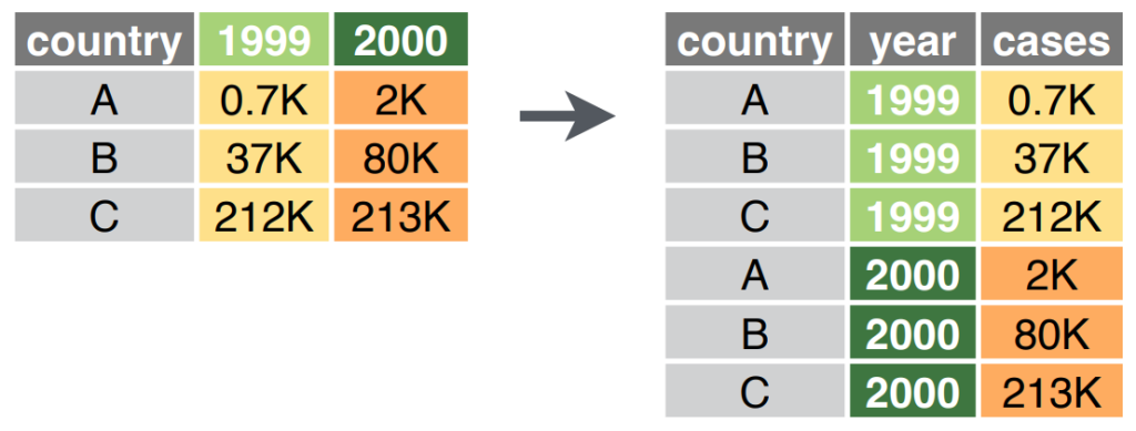
Pivot Longer

Pivot longer transforms wide data into long data by collapsing multiple columns into two new columns: one for the variable names and one for their values. This is particularly useful when you have repeated measurements or multiple variables stored in column names.

Let’s start with a dataset for this:

df_wide_eco <- tibble(
  # Plot information
  plot_id = paste0("Plot", str_pad(1:6, 2, pad = "0")),
  plot_type = rep(c("Control", "Treatment"), 3),
  elevation = round(rnorm(6, mean = 500, sd = 50), 0), # meters

  # Quercus rubra measurements for 2020-2022
  Q_rubra_height_2020 = round(rnorm(6, mean = 15, sd = 2), 1),
  Q_rubra_height_2021 = round(rnorm(6, mean = 16, sd = 2), 1),
  Q_rubra_height_2022 = round(rnorm(6, mean = 17, sd = 2), 1),
  Q_rubra_dbh_2020 = round(rnorm(6, mean = 30, sd = 5), 1),
  Q_rubra_dbh_2021 = round(rnorm(6, mean = 32, sd = 5), 1),
  Q_rubra_dbh_2022 = round(rnorm(6, mean = 34, sd = 5), 1),

  # Acer saccharum measurements for 2020-2022
  A_saccharum_height_2020 = round(rnorm(6, mean = 12, sd = 1.5), 1),
  A_saccharum_height_2021 = round(rnorm(6, mean = 13, sd = 1.5), 1),
  A_saccharum_height_2022 = round(rnorm(6, mean = 14, sd = 1.5), 1),
  A_saccharum_dbh_2020 = round(rnorm(6, mean = 25, sd = 4), 1),
  A_saccharum_dbh_2021 = round(rnorm(6, mean = 27, sd = 4), 1),
  A_saccharum_dbh_2022 = round(rnorm(6, mean = 29, sd = 4), 1),

  # Betula alleghaniensis measurements for 2020-2022
  B_alleghaniensis_height_2020 = round(rnorm(6, mean = 18, sd = 2.5), 1),
  B_alleghaniensis_height_2021 = round(rnorm(6, mean = 19, sd = 2.5), 1),
  B_alleghaniensis_height_2022 = round(rnorm(6, mean = 20, sd = 2.5), 1),
  B_alleghaniensis_dbh_2020 = round(rnorm(6, mean = 35, sd = 6), 1),
  B_alleghaniensis_dbh_2021 = round(rnorm(6, mean = 37, sd = 6), 1),
  B_alleghaniensis_dbh_2022 = round(rnorm(6, mean = 39, sd = 6), 1)
)
df_wide_eco

# A tibble: 6 × 21
  plot_id plot_type elevation Q_rubra_height_2020 Q_rubra_height_2021 Q_rubra_height_2022 Q_rubra_dbh_2020 Q_rubra_dbh_2021 Q_rubra_dbh_2022 A_saccharum_height_2020 A_saccharum_height_2021 A_saccharum_height_2022 A_saccharum_dbh_2020 A_saccharum_dbh_2021 A_saccharum_dbh_2022 B_alleghaniensis_height_2020 B_alleghaniensis_heigh…¹ B_alleghaniensis_hei…² B_alleghaniensis_dbh…³ B_alleghaniensis_dbh…⁴
  <chr>   <chr>         <dbl>               <dbl>               <dbl>               <dbl>            <dbl>            <dbl>            <dbl>                   <dbl>                   <dbl>                   <dbl>                <dbl>                <dbl>                <dbl>                        <dbl>                    <dbl>                  <dbl>                  <dbl>                  <dbl>
1 Plot01  Control         490                15.8                15.1                17               32.4             28.8             30.1                    11                      12.2                    13.4                 32.1                 36.6                 30.2                         12.4                     17.4                   23.6                   41.7                   40.1
2 Plot02  Treatment       533                13.1                17.7                13.4             36.9             21.2             38.2                    12                      13.3                    10                   26.1                 27                   25                           21.1                     19.4                   22.6                   32.1                   34.7
3 Plot03  Control         514                16.7                17                  17.1             32.3             36.4             27.7                    13                      13.7                    13.9                 25.5                 33.5                 29.1                         14.9                     20.1                   21.1                   36.4                   30.4
4 Plot04  Treatment       551                14.1                14.8                17.4             24.3             27.9             32.2                     9.5                    13.4                    14.6                 30.1                 21.2                 24.7                         19.1                     21.2                   21.8                   33.2                   44.3
5 Plot05  Control         541                19.8                14                  17.3             27.8             29.1             33.6                    11.5                    14                      14.8                 22.1                 26.2                 31.9                         19.6                     13.9                   22.3                   40.2                   41.4
6 Plot06  Treatment       490                11.7                16.3                14.9             31.7             39.5             28.2                    13.1                    12.8                    13.2                 23.2                 28.5                 33.3                         17.5                     14.9                   13.3                   32.9                   47.3
# ℹ abbreviated names: ¹​B_alleghaniensis_height_2021, ²​B_alleghaniensis_height_2022, ³​B_alleghaniensis_dbh_2020, ⁴​B_alleghaniensis_dbh_2021
# ℹ 1 more variable: B_alleghaniensis_dbh_2022 <dbl>

The basic syntax of pivot_longer requires three main arguments:

• cols: Specifies which columns to pivot (can use tidyselect helpers like starts_with())
• names_to: The name of the new column that will contain the old column names
• values_to: The name of the new column that will contain the values

Example 1: Basic Pivot Longer

df_long_simple <- df_wide_eco %>%
  pivot_longer(
    cols = starts_with(c("Q_", "A_", "B_")),
    names_to = "target",
    values_to = "value"
  )
df_long_simple

# A tibble: 108 × 5
   plot_id plot_type elevation target                  value
   <chr>   <chr>         <dbl> <chr>                   <dbl>
 1 Plot01  Control         490 Q_rubra_height_2020      15.8
 2 Plot01  Control         490 Q_rubra_height_2021      15.1
 3 Plot01  Control         490 Q_rubra_height_2022      17  
 4 Plot01  Control         490 Q_rubra_dbh_2020         32.4
 5 Plot01  Control         490 Q_rubra_dbh_2021         28.8
 6 Plot01  Control         490 Q_rubra_dbh_2022         30.1
 7 Plot01  Control         490 A_saccharum_height_2020  11  
 8 Plot01  Control         490 A_saccharum_height_2021  12.2
 9 Plot01  Control         490 A_saccharum_height_2022  13.4
10 Plot01  Control         490 A_saccharum_dbh_2020     32.1
# ℹ 98 more rows

In this example, we’ve taken all columns that start with “Q_”, “A_”, or “B_” (our species measurements) and collapsed them into two new columns: “target” (containing the original column names) and “value” (containing the measurements). This gives us a long-format dataset where each row represents a single measurement.

The names_sep argument allows us to split the column names into multiple columns based on a delimiter. This is useful when your column names contain multiple pieces of information separated by a character (like an underscore).

Example 2: Using names_sep to pivot longer & splitting the singular collapsed column into multiple

df_long_split <- df_wide_eco %>%
  pivot_longer(
    cols = starts_with(c("Q_", "A_", "B_")),
    names_sep = "_",
    names_to = c("genus_letter", "species_code", "measurement_type", "survey_year"),
    values_to = "measurement_value"
  )
df_long_split

# A tibble: 108 × 8
   plot_id plot_type elevation genus_letter species_code measurement_type survey_year measurement_value
   <chr>   <chr>         <dbl> <chr>        <chr>        <chr>            <chr>                   <dbl>
 1 Plot01  Control         490 Q            rubra        height           2020                     15.8
 2 Plot01  Control         490 Q            rubra        height           2021                     15.1
 3 Plot01  Control         490 Q            rubra        height           2022                     17  
 4 Plot01  Control         490 Q            rubra        dbh              2020                     32.4
 5 Plot01  Control         490 Q            rubra        dbh              2021                     28.8
 6 Plot01  Control         490 Q            rubra        dbh              2022                     30.1
 7 Plot01  Control         490 A            saccharum    height           2020                     11  
 8 Plot01  Control         490 A            saccharum    height           2021                     12.2
 9 Plot01  Control         490 A            saccharum    height           2022                     13.4
10 Plot01  Control         490 A            saccharum    dbh              2020                     32.1
# ℹ 98 more rows

Here, we’ve used names_sep = "_" to split the column names at each underscore, creating four new columns: “genus_letter” (Q, A, B), “species_code” (rubra, saccharum, alleghaniensis), “measurement_type” (height, dbh), and “survey_year” (2020, 2021, 2022). This gives us a much more structured dataset where each piece of information from the column names is in its own column.

The names_pattern argument provides even more control over how column names are split. It uses regular expressions (regex) to extract specific parts of the column names. This is particularly useful when your column names follow a complex pattern or when you need more precise control over the splitting.

Example 3: Using names_pattern to perform a more fine-tuned splitting on the singular collapsed column

df_long_pattern <- df_wide_eco %>%
  pivot_longer(
    cols = starts_with(c("Q_", "A_", "B_")),
    names_to = c("sample_name", "measurement_type", "survey_year"),
    names_pattern = "([A-Z]_[a-z]+)_([a-z]+)_(\\d{4})",
    values_to = "measurement_value"
  )
df_long_pattern

# A tibble: 108 × 7
   plot_id plot_type elevation sample_name measurement_type survey_year measurement_value
   <chr>   <chr>         <dbl> <chr>       <chr>            <chr>                   <dbl>
 1 Plot01  Control         490 Q_rubra     height           2020                     15.8
 2 Plot01  Control         490 Q_rubra     height           2021                     15.1
 3 Plot01  Control         490 Q_rubra     height           2022                     17  
 4 Plot01  Control         490 Q_rubra     dbh              2020                     32.4
 5 Plot01  Control         490 Q_rubra     dbh              2021                     28.8
 6 Plot01  Control         490 Q_rubra     dbh              2022                     30.1
 7 Plot01  Control         490 A_saccharum height           2020                     11  
 8 Plot01  Control         490 A_saccharum height           2021                     12.2
 9 Plot01  Control         490 A_saccharum height           2022                     13.4
10 Plot01  Control         490 A_saccharum dbh              2020                     32.1
# ℹ 98 more rows

In this example, we’ve used a regular expression pattern to extract three groups from the column names: the species name (e.g., “Q_rubra”), the measurement type (e.g., “height”), and the year (e.g., “2020”). The pattern ([A-Z]_[a-z]+)_([a-z]+)_(\\d{4}) breaks down as:

• ([A-Z]_[a-z]+) – First group: A capital letter followed by an underscore and lowercase letters (species name)
• _([a-z]+)_ – Second group: An underscore, lowercase letters, and another underscore (measurement type)
• (\\d{4}) – Third group: Four digits (year)

This gives us more control over how the column names are split compared to names_sep, allowing us to keep the species name as a single column rather than splitting it into genus and species.

It is understandable that regular expressions can feel like an alien language at this point for you. Fortunately, if you have the time, there are fantastic resources online such as this start-to-finish tutorial that will get you familiar with regular expressions in no time!

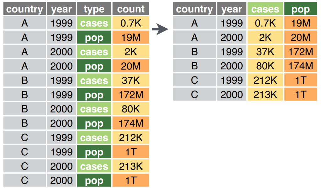
Pivot Wider

Pivot wider is the opposite of pivot longer – it transforms long data into wide data by spreading a column of variable names into multiple columns. This is useful when you want to create a summary table or when you need to prepare data for certain types of analysis.

We’ll make a dataset for this:

df_long_eco <- tibble(
  plot_id = rep(paste0("Plot", str_pad(1:4, 2, pad = "0")), each = 9), # 4 plots × 3 species × 3 years
  species = rep(rep(c("Quercus rubra", "Acer saccharum", "Betula alleghaniensis"), each = 3), 4),
  year = rep(2020:2022, 12), # 12 combinations of plot × species
  height = round(rnorm(36, mean = 15, sd = 2), 1), # Height in meters
  dbh = round(rnorm(36, mean = 30, sd = 5), 1), # Diameter at breast height in cm
  leaf_area = round(rnorm(36, mean = 100, sd = 15), 1) # Leaf area in cm²
)
df_long_eco

# A tibble: 36 × 6
   plot_id species                year height   dbh leaf_area
   <chr>   <chr>                 <int>  <dbl> <dbl>     <dbl>
 1 Plot01  Quercus rubra          2020   14.3  28.9      92.2
 2 Plot01  Quercus rubra          2021   15.2  30.8     110. 
 3 Plot01  Quercus rubra          2022   18.2  35.8      99.1
 4 Plot01  Acer saccharum         2020   14.8  35.3     110. 
 5 Plot01  Acer saccharum         2021   17.2  35.7     120  
 6 Plot01  Acer saccharum         2022   16.3  27.1     100. 
 7 Plot01  Betula alleghaniensis  2020   14.8  40       115. 
 8 Plot01  Betula alleghaniensis  2021   11.9  30.3      82.2
 9 Plot01  Betula alleghaniensis  2022   14    39.3      89.2
10 Plot02  Quercus rubra          2020   14    23.2     123. 
# ℹ 26 more rows

# A tibble: 12 × 5
   plot_id species               height_2020 height_2021 height_2022
   <chr>   <chr>                       <dbl>       <dbl>       <dbl>
 1 Plot01  Quercus rubra                14.3        15.2        18.2
 2 Plot01  Acer saccharum               14.8        17.2        16.3
 3 Plot01  Betula alleghaniensis        14.8        11.9        14  
 4 Plot02  Quercus rubra                14          15.1        17.6
 5 Plot02  Acer saccharum               19.6        18.1        14.7
 6 Plot02  Betula alleghaniensis        11.5        14.2        15.2
 7 Plot03  Quercus rubra                16.7        16.9        16.4
 8 Plot03  Acer saccharum               12.2        16.7        14.1
 9 Plot03  Betula alleghaniensis        15.3        15.1        15.9
10 Plot04  Quercus rubra                15          11.7        16.5
11 Plot04  Acer saccharum               15.8        14.5        15.2
12 Plot04  Betula alleghaniensis        15.3        15.4        18.3

The pivot_wider function requires at least two main arguments:

• names_from: The column whose values will become the new column names
• values_from: The column whose values will fill the new columns

Example 1: Basic pivot_wider.

df_wide_basic <- df_long_eco %>%
  select(plot_id, species, year, height) %>%
  pivot_wider(
    names_from = year,
    values_from = height,
    names_prefix = "height_"
  )
df_wide_basic

In this example, we’ve taken the “year” column and used its values (2020, 2021, 2022) to create new column names, prefixed with “height_”. The values from the “height” column are then placed in these new columns. This gives us a wide-format dataset where each row represents a unique combination of plot and species, and the columns represent height measurements for each year.

The names_glue argument provides a template for creating the new column names. It uses a special syntax where {.value} is replaced with the name of the value column, and any other column names in curly braces are replaced with their values. This is particularly useful when you have multiple value columns and want to create more descriptive column names.

Example 2: Using names_glue.

df_wide_glue <- df_long_eco %>%
  pivot_wider(
    id_cols = c(plot_id, species),
    names_from = year,
    values_from = c(height, dbh, leaf_area),
    names_glue = "{.value}_{year}"
  )
df_wide_glue

# A tibble: 12 × 11
   plot_id species               height_2020 height_2021 height_2022 dbh_2020 dbh_2021 dbh_2022 leaf_area_2020 leaf_area_2021 leaf_area_2022
   <chr>   <chr>                       <dbl>       <dbl>       <dbl>    <dbl>    <dbl>    <dbl>          <dbl>          <dbl>          <dbl>
 1 Plot01  Quercus rubra                14.3        15.2        18.2     28.9     30.8     35.8           92.2          110.            99.1
 2 Plot01  Acer saccharum               14.8        17.2        16.3     35.3     35.7     27.1          110.           120            100. 
 3 Plot01  Betula alleghaniensis        14.8        11.9        14       40       30.3     39.3          115.            82.2           89.2
 4 Plot02  Quercus rubra                14          15.1        17.6     23.2     30.1     36.2          123.           106.            69.2
 5 Plot02  Acer saccharum               19.6        18.1        14.7     26.4     26.2     25.3           79.5           97            113  
 6 Plot02  Betula alleghaniensis        11.5        14.2        15.2     24.7     27.8     31.7           98.5          109.           114. 
 7 Plot03  Quercus rubra                16.7        16.9        16.4     19.9     31.1     36.2          125.           101.            99.2
 8 Plot03  Acer saccharum               12.2        16.7        14.1     40.2     36.5     33.8           73.7          102.            91.4
 9 Plot03  Betula alleghaniensis        15.3        15.1        15.9     21.4     27       28.2           85.4           97.3          115. 
10 Plot04  Quercus rubra                15          11.7        16.5     33.5     29.5     23.7           70.1           93.6          102. 
11 Plot04  Acer saccharum               15.8        14.5        15.2     38.4     34.6     31.2           86.6          105            106. 
12 Plot04  Betula alleghaniensis        15.3        15.4        18.3     36.1     23.3     33.3           99.5           63            139. 

In this example, we’ve used names_glue = "{.value}_{year}" to create column names that combine the value column name (height, dbh, or leaf_area) with the year. This gives us a wide-format dataset with columns like “height_2020”, “dbh_2020”, “leaf_area_2020”, etc. The id_cols argument specifies which columns should remain as identifiers (plot_id and species in this case).

Summary

Data reshaping is a fundamental skill in ecological data analysis. By mastering pivot_longer and pivot_wider, you can:

• Transform data between wide and long formats to suit different analytical needs
• Extract information embedded in column names into separate columns
• Create summary tables with measurements across time points or treatments
• Prepare data for visualization with ggplot2 or statistical analysis

Remember that tidy data principles guide these operations: each variable should form a column, each observation should form a row, and each type of observational unit should form a table. By reshaping your data appropriately, you can make your analyses more straightforward and your code more readable.